Lin Wang and Guixian Tian
Empirical Research on the Relationship between the Futures and Spot Prices of Cotton in China
Abstract: This study constructed a VAR model with cotton futures and spot price data from April 30, 2009 to November 16, 2022, for empirical analysis utilizing the Granger causality test to analyze the dynamic relationship between cotton futures and spot market prices in China. The impulse response function and variance decomposition analysis showed that the cotton spot prices at flowering have a causal relationship with each other; in terms of mutual influence and impact, futures prices are higher than spot prices. Finally, it proposed countermeasures and suggestions from the perspective of establishing a standardized cotton spot market, improving the laws and regulations of the cotton futures market and trading system, and optimizing the structure of investment subjects.
Keywords: Cotton Futures Price , Cotton Spot Price , Spot Market , VAR
1. Introduction
Cotton is China's most significant economic crop; it is not only the raw material of the textile industry but also crucial to the chemical industry and is of vital importance to the nation's economy and people's livelihoods. Although China is a large cotton-producing and a large cotton-consuming country, it has no say in the global pricing of cotton, which makes its industry vulnerable to the risks brought about by global cotton price fluctuations. Cotton futures were officially listed on the Zhengzhou Commodity Exchange on June 1, 2004, opening the curtain for the coordinated development of cotton futures and spot markets to stabilize cotton prices and enhance the influence of Chinese cotton prices worldwide. Since listing cotton futures over 18 years ago, it has played a significant role in helping cotton farmers and industrial chain enterprises find prices and avoid risks. However, since 2020, the pandemic has spread globally, and economic and trade friction between China and the United States has intensified. Multiple factors overlap, and cotton price volatility intensifies. To understand whether the futures market is able to find the price and avoid risk and to study the price correlation degree of China's cotton futures and spot markets, this study empirically examines cotton prices from the perspective of the correlation between cotton futures and spot prices and discusses the transmission relationship.
Between cotton futures and spot prices, this study analyzes the transmission connection, which is helpful in finding out the formation mechanism and changing the law of cotton futures and spot prices in China, providing reference for cotton agricultural production, cotton futures investment and further development of the market.
2. Literature Review
International academics have extensively researched the connection between futures and spot prices for various products. Sims [1] first proposed using the VAR model to study the connection between spot and futures prices, which can treat both prices as endogenous variables and reduce the inaccuracy caused by the subjective estimation of the determining relationship. Brooks et al. [2] simultaneously used VAR and vector error correction model (VECM) models to conduct an empirical analysis of the connection between spot prices for FTSE-100 index futures and concluded that the lag change in futures prices can be used to predict how spot prices will fluctuate. Sanjay et al. [3] used the generalized autoregressive conditional heteroskedasticity model (GARCH-BEEK) model to perform a dynamic analysis of the futures and spot prices in the four foreign exchange markets of the National Stock Exchange of India and the Commodities Exchange, finding a correlation between Indian foreign currency futures prices and spot prices; short-term changes in futures prices would create fluctuations in spot prices, and long-term changes in the latter would have an effect on the former.
Many domestic scholars have conducted qualitative and quantitative analyses of the relationship between futures and spot prices. For example, Chen and Zou [4] used the Johanson cointegration test, Granger causality analysis, and bivariate exponential generalized autoregressive conditional heteroskedasticity (EC-EGARCH) model to conduct empirical research on the connection between corn futures spot prices, and they came to the conclusion that there was a cointegration relationship and a causal guidance relationship between corn futures spot prices. Sui and Zhang [5] used the cointegration test, Granger causality test, error correlation model, and impulse response function to study the dynamic correlation between the spot prices of thermal coal. They concluded that there is a long-term cointegration connection between the two prices and that the futures price has a guiding effect on the spot price, but the latter has no guiding effect on the former. Ji and Rui [6] constructed a VAR model to explore whether there is a linkage relationship between the spot price of gold futures and empirically prove that the futures price has a one-way impact on the market price of gold and that the futures price is unaffected by the actual price.
Finally, numerous academics have investigated the connection between spot and futures prices; the research objects mainly focus on metal products; research on agricultural products is relatively small, and research on cotton in agricultural products is even less. Therefore, this study examines the dynamic relationship between the cotton futures market and spot market prices in China and analyzes the connection between them in depth.
3. VAR Model and Estimation Method
VAR, whose full name is the vector autoregressive model, was proposed by macroeconomist Sims [1] in 1980 as an unstructured multi-equation model. VAR bases model construction on the statistical structure of the data, not on economic theory. Therefore, building a VAR model does not need to be based on economic theory but rather on the information provided by the time series of economic indicators to verify the theoretical relationship between the economic variables.
Expression of the VAR model:
(1)
[TeX:] $$Y_t=\mathrm{c}+\alpha_1 Y_{t-1}+\alpha_2 Y_{t-2}+\alpha_3 Y_{t-3}+\cdots, \alpha_k Y_{t-k}+\mu$$Among them, [TeX:] $$Y_t=\left(y_{1, t}, y_{2, t}, \ldots, y_{N, t}\right)^{\prime} .$$
(3)
[TeX:] $$\alpha_j=\left(\begin{array}{cccc} \alpha_{11 . j} &\alpha_{12 . j} &\cdots &\alpha_{1 N . j} \\ \alpha_{21 . j} &\alpha_{22 . j} &\cdots &\alpha_{2 N . j} \\ \vdots &\vdots &\cdots &\vdots \\ \alpha_{N 1 . j} &\alpha_{N 2 . j} &\cdots &\alpha_{N N . j} \end{array}\right), j=1,2, \ldots, k,$$
This is a VAR model containing N variables with lag k. [TeX:] $$Y_t$$ denotes the N×1st order endogenous variable vector, [TeX:] $$\alpha_i$$ is the N×Nth-order matrix of the ith parameter to be estimated, and [TeX:] $$\mu_t$$ is the N×1st order random error column vector.
4. Variable Selection and Descriptive Statistics
4.1 Variable Selection
In this study, the cotton spot price data were selected as the daily transaction average price, cotton futures price data were selected as the daily active contract closing price, and the selected sample interval was from April 30, 2009 to November 16, 2022, all from the wind database. Due to the non-daily continuity of futures trading, the period spot price cannot be fully corresponded to; this study eliminated holidays and weekends that did not correspond to the missing number and finally obtained 3,283 groups of data.
This study used the software Eviews8.0 for data processing and analysis. This study used these two groups of data to conduct an empirical analysis of the connection between the current cotton spot price and cotton futures price in China through the cotton futures and spot price trend chart (Fig. 1), which shows that the trends of cotton futures and spot prices are basically the same. The cycle of change is basically the same.
4.2 Description of Data Statistics
All the data of the two sets were taken as logarithms to decrease the heteroskedasticity and volatility of the two time-series datasets: the Chinese cotton futures price corresponds to LnCF, and the Chinese cotton spot price corresponds to LnCP. Table 1 presents the descriptive results of the two prices series. As demonstrated by Table 1, the skewness coefficients of both series were positive, and both distributions were right-skewed; the peaks were greater than 3, and both distributions have the characteristics of cusp distribution. At the same time, the J-B statistical test was significant, demonstrating that neither of the series is normally distributed. In summary, the data characteristics and distributions of the two series are very similar.
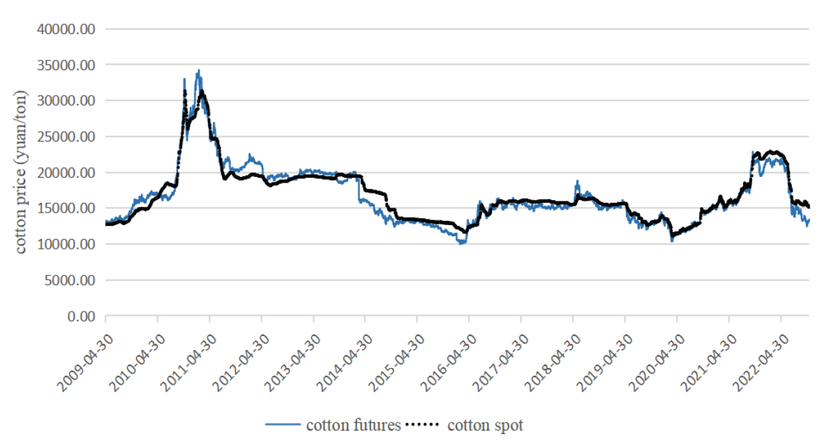
Table 1.
| Statistical quantity | LnCF | LnCP |
|---|---|---|
| Average value | 9.6945 | 9.7102 |
| Median | 9.6496 | 9.6761 |
| Maximum value | 10.4413 | 10.3527 |
| Minimum value | 9.2093 | 9.3154 |
| Standard deviation | 0.2248 | 0.2070 |
| Skewness | 0.6021 | 0.6698 |
| Kurtosis | 3.2435 | 3.3275 |
| J-B statistic | 206.4675 | 260.1239 |
| P-value | 0.0000 | 0.0000 |
5. Empirical Analysis
A VAR model was established to empirically investigate the association between cotton futures and spot prices. First, the augmented Dickey–Fuller (ADF) test was used to check if there is a unit root in the two prices series and to determine the stationarity of the two variables; then, the lag order was determined, and the VAR model was established. Then, the stability of the model was tested, and analysis of the Granger causality test, impulse response function and variance decomposition were performed in turn after the test to observe the mutual influence and effect between the two pairs of prices.
5.1 ADF Inspection
To avoid the problem of "pseudo-regression" due to the non-smoothness of the time-series variables, it is necessary to judge the smoothness and non-smoothness of the time series of the two variables before building the model. ADF was used to examine the stationarity of the LnCF and LnCP variables, and Table 2 presents the test findings. The test results showed that the cotton spot price and cotton futures series are both nonstationary series with a unit root; however, the first-order difference series is stationary and does not have a unit root. Therefore, both the cotton futures and spot prices are first-order singleinteger series that satisfy the subsequent modeling and a series of test conditions.
Table 2.
| Variable | ADF value | ADF test threshold | P-value | Result | ||
|---|---|---|---|---|---|---|
| 1% level | 5% level | 10% level | ||||
| LnCF | -1.719535 | -3.43215 | -2.86222 | -2.56718 | 0.4213 | Unstable |
| LnCP | -2.03406 | -3.43215 | -2.86222 | -2.56717 | 0.2723 | Unstable |
| D(LnCF) | -57.43700 | -3.43215 | -2.86222 | -2.56718 | 0.0001 | Stable |
| D(LnCP) | -15.30887 | -3.43216 | -2.86222 | -2.56718 | 0.0000 | Stable |
5.2 Building a VAR Model
From the previous analysis, it can be seen that LnCF and LnCP are first-order single integer series; if the original data are directly used to construct the VAR model, it will make the model unstable while the impulse response function will not converge, resulting in the loss of significance of the impulse response function analysis; therefore, the first-order difference data were used to construct the VAR model in this study.
First, the lag order was determined. Before building the VAR model, the LR and LL statistics and the final prediction error (FPE), Akaike information criterion (AIC), Schwarz criterion (SC), and Hannan- Quinn criterion (HQ) criteria were applied to determine the lag order of the model. The optimal lag order was determined to be five periods according to the criterion of the majority of lag terms (Table 3).
Second, the stationarity test for the model was conducted. The stability of the model must be tested to ensure that it is valid and that the impulse response function and variance decomposition that follow are meaningful. Fig. 2 depicts the test findings in which the unit roots are all contained within a circle, proving that the established VAR model is stable.
Table 3.
| Lag | LogL | LR | FPE | AIC | SC | HQ |
|---|---|---|---|---|---|---|
| 0 | 22326.07 | NA | 4.15e-09 | -13.62470 | -13.62098 | -13.62337 |
| 1 | 23132.52 | 1611.424 | 2.54e-09 | -14.11445 | -14.10329 | -14.11045 |
| 2 | 23256.38 | 247.3409 | 2.36e-09 | -14.18760 | -14.16900 | -14.18094 |
| 3 | 23281.44 | 50.01399 | 2.33e-09 | -14.20045 | -14.17441 | -14.19113 |
| 4 | 23293.25 | 23.55928 | 2.32e-09 | -14.20522 | -14.17174 | -14.19323 |
| 5 | 23318.39 | 50.11828* | 2.29e-09* | -14.21812* | -14.17721* | -14.20347* |
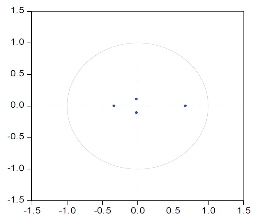
Table 4.
| Lag period | Original hypothesis | F-value | P-value | Conclusion |
|---|---|---|---|---|
| 5 | Granger's reason why D (LnCF) is not D (LnCP) | 143.998 805 | 0.0000 | Rejection |
| Granger's reason why D (LnCP) is not D (LnCF) | 3.898 383 | 0.0015 | Rejection |
5.3 Granger Causality Test
The VAR model tests the causal connection between each time-series variable. To further analyze the interdependence between variables and discuss whether cotton futures and spot prices are causally related to each other, this study used Granger causality; Table 4 displays the test findings. As demonstrated in Table 4, the original hypothesis was rejected at the 1% significance level; that is, cotton futures and spot prices are causally related. The conclusion that cotton futures prices are causally related is valid and that cotton futures price movements have a more pronounced impact on spot prices.
5.4 Impulse Response Function
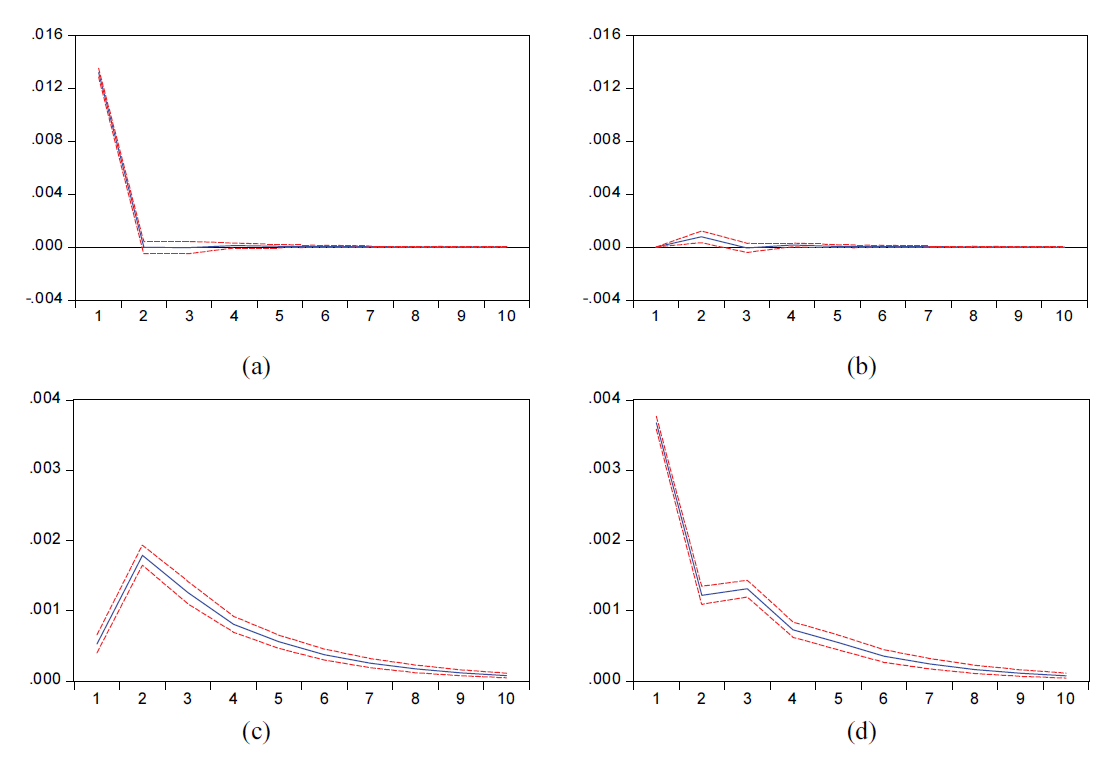
Establishing a VAR model combined with the above test results showed that cotton spot prices and cotton futures prices have a causal link but do not reflect the mutual influence between the two prices. Next, this study based on the above VAR model of the two prices' impulse response function, analyzed and investigated the dynamic effects of the price connection between the two; Fig. 3 displays the test findings.
As can be seen from Fig. 3, given a standard deviation information shock to the cotton futures price, the cotton futures price, on their own price shock impact, initially had a 1.3% growth response. In the 2nd period, the impact gradually converged, and from the 2nd to the 10th period, it ceased to have an impact. The cotton spot price from the cotton futures price shock in the 1st period only began to have a response. In the 2nd period, the response reached the maximum, with a growth response of approximately 0.2%. Then, the degree of response slowly decreased, with the impact slowly disappearing from the 9th period onwards. Conversely, when a positive shock is given to the cotton spot price, the cotton futures price responds to the shock from the cotton spot price only after the 1st period, with the maximum impact in the 2nd period, followed by a positive and negative impact, which gradually disappears from the 4th period; The cotton spot price responds to its own shock to a greater extent, reaching a peak in the 1st period, with a response of 0.0038. It then started to fall, there was a slow rise in the 3rd period, and the impact slowly disappeared. This indicates that the transmission of price shocks from the cotton futures market to the spot market is faster, and the degree of response is greater, whereas the transmission from the spot market to the futures market is slower, and the degree of response is smaller.
Fig. 3.
5.5 Analysis of Variance Decomposition
The previous impulse response function shows the response of the two variables of cotton futures and spot prices in the face of shocks, but the degree of impact of shocks cannot be quantified. Thus, the variance decomposition analysis of the VAR can observe the degree of contribution of each variable, and the contribution rate is shown in Table 5.
It can be seen that with a gradual increase in the number of periods combined with the data in Table 5, the contribution of the cotton spot price to the cotton futures price gradually increases. However, the overall contribution is very small. It does not exceed 1%, indicating that the price of cotton futures is mainly influenced by its own price changes, and the degree of influence has been maintained at more than 99%. Looking at the cotton spot price, in addition to the impact of their own factors, but also by the impact of futures price shocks, with the increase in the number of periods, the degree of influence of the variance of the cotton spot price of its own changes gradually weakened; the contribution rate fell from 97.96% to 73.84%, while the degree of influence of the variance of the cotton futures price changes increased, from 2.04% to 26.16%. The above analysis shows that the degree of influence of cotton futures prices on cotton spot prices is much greater than that of the latter on the former; China's cotton spot price is more influenced by cotton futures prices.Table 5.
| Period | D(LNCF) variance decomposition | D(LNCP) variance decomposition | ||
|---|---|---|---|---|
| D(LNCF) | D(LNCP) | D(LNCF) | D(LNCP) | |
| 1 | 100 | 0 | 2.035847 | 97.964153 |
| 2 | 99.656107 | 0.343893 | 18.882278 | 81.117722 |
| 3 | 99.653491 | 0.346509 | 23.283661 | 76.716339 |
| 4 | 99.640522 | 0.359478 | 24.925414 | 75.074586 |
| 5 | 99.639563 | 0.360437 | 25.602756 | 74.397244 |
| 6 | 99.638241 | 0.361759 | 25.910721 | 74.089276 |
| 7 | 99.637857 | 0.362143 | 26.049016 | 73.950984 |
| 8 | 99.637632 | 0.362368 | 26.112686 | 73.887314 |
| 9 | 99.637539 | 0.362461 | 26.141892 | 73.858108 |
| 10 | 99.637494 | 0.362506 | 26.155366 | 73.844634 |
6. Summary and Suggestions
Through empirical research on the dynamic connection between China's cotton futures and spot price, it was found that cotton futures and spot prices affect each other; however, the mutual guidance of the two is uneven, the transmission of the spot price to the futures price is weak, and the futures price is mainly affected by its own price changes. The futures price over a long period influences the cotton spot price. In short, the cotton futures market is a price discovery function to a certain extent; however, the strength of the cotton spot market in terms of futures price transmission is insufficient. In this regard, the following countermeasures and suggestions are proposed.
First, a standardized cotton spot market should be established. The transmission effect of cotton from the spot market to the futures market is less effective than the impact of the latter on the former; it may be that China's cotton spot market development is not perfect, the market trading body behavior is not sufficiently standardized, and spot market price fluctuations cannot be effectively transmitted to the futures market. In this regard, the government can integrate cotton markets in various regions and establish a standardized and unified spot market for cotton trading units, trading contracts, quality, and other aspects of standardized regulations and improve the spot market cotton quality inspection system so that its standards and futures market inspection standards make the spot market and futures market form an organic market system.
Second, the laws and regulations regarding the cotton futures market should be improved. China's cotton futures market started later than developed countries such as Europe and the United States, and the relevant legal system, management, system, and other aspects are not perfect. In this regard, regulatory authorities need to relax control of the cotton futures market, and the government needs to improve relevant laws and regulations as soon as possible to ensure the healthy and orderly development of the cotton futures market.
Third, the structure of the main body of investment should be optimized to encourage cotton farmers to become the main body of futures market transactions. Thus far, China's cotton futures market investment subjects are mainly institutional investors and some retail investors with capital, whereas, in the United States, one-third of the farmers directly or indirectly use the cotton futures market to hedge risk. In addition to the lack of professional futures expertise of China's cotton farmers, there is a lack of industrialization of cotton development, cotton cultivation is more dispersed in family-based units, and cotton production makes it difficult to reach the futures market with a contract specified in 5 tons/hand. Therefore, the structure of the main investment body should be optimized to encourage cotton farmers to participate in future market transactions. On the one hand, China should strengthen the training of cotton farmers' future knowledge, and on the other hand, the development of China's cotton industrialization should be accelerated.
Biography

References
- 1 C. A. Sims, "Macroeconomics and reality," Econometrica, vol. 48, no. 1, pp. 1-48, 1980. https://doi.org/10.2307/1912017doi:[[[10.2307/191]]]
- 2 C. Brooks, A. G. Rew, and S. Ritson, "A trading strategy based on the lead–lag relationship between the spot index and futures contract for the FTSE 100," International Journal of Forecasting, vol. 17, no. 1, pp. 31-44, 2001. https://doi.org/10.1016/S0169-2070(00)00062-5doi:[[[10.1016/S0169-(00)00062-5]]]
- 3 S. Sehgal, W. Ahmad, and F. Deisting, "An investigation of price discovery and volatility spillovers in India’s foreign exchange market," Journal of Economic Studies, vol. 42, no. 2, pp. 261-284, 2015. https://doi.org/10.1108/JES-11-2012-0157doi:[[[10.1108/JES-11--0157]]]
- 4 B. J. Chen and H. R. Zou, "Empirical analysis of correlation fluctuations between China’s corn futures and spot prices," Enterprise Economy, vol. 32, no. 4, pp. 178-182, 2013.custom:[[[-]]]
- 5 G. L. Sui and G. H. Zhang, "Research on the dynamic relationship between thermal coal futures prices and spot prices," China Coal, vol. 41, no. 5, pp. 5-10, 2015. https://doi.org/10.3969/j.issn.1006-530X.2015.05.001doi:[[[10.3969/j.issn.1006-530X.2015.05.001]]]
- 6 C. J. Ji and L. R. Rui, "China's gold futures based on V AR model Analysis of price and spot price linkage," Market Weekly, vol. 34, no. 6, pp. 132-135, 2021.custom:[[[-]]]