Zhi-lai Zhang , Shao-jun Jiang and Li-li Liang
Analysis of DDS Sampling Method and Harmonic Composition
Abstract: Through theoretical proof and algorithm design, this paper numerically demonstrates that the three sampling methods of DDS are equivalent in amplitude-frequency characteristics. Depending on theoretical analysis, the article obtains the conclusion that 2 points are optimal when sampling at 2, 3, and 4 points. Built on the data results, this paper obtains the fractional form of the amplitude and phase of the DDS sampled signal; in addition, this paper also obtains the design parameters of the DDS post-stage filter. It also gives a control method for the calculation error when addressing this issue.
Keywords: DDS , Fourier series , Numerical Analysis
1. Introduction
Using a sine sampling table and a low-pass filter to produce a sine wave is an important technology to generate a sine wave [1]. This method has significant applications in direct digital frequency synthesis (DDS) and forced pulse width modulation (FPWM). From the public information, low-pass filter theory and practical tools are very mature; however, there are few studies on the sampling method and signal spectrum of DDS sinusoidal signals. Some documents analyze the DDS output signal spectrum, but the final result is in the form of the cumulative sum of infinite sampling signals [2,3]. Since the DDS post-stage still needs filtering [4]; obviously, this form does not make much sense for follow-up work. But in fact, for the digital-to-analog (DA) sampling mode, for the parameters of the low-pass filter, this question has important meaning [5-7]. What is the relationship between the sampling method and the filter parameters? Is there any other better sampling table? This paper focuses on computational simulation research on this problem.
This article consists of four parts. The first part of this article takes the 2-point DA sine fitting signal as an example. Through the demonstration of the fast Fourier transform (FFT) algorithm data, it proves that the FFT is unreasonable for this analysis. In the second part, through theoretical derivation and algorithm description, spectrum publicity suitable for formula is obtained. The third part uses this formula to complete the comparative analysis of three different sampling methods. The fourth part briefly describes the conclusion and the problem to be resolved.
2. Traditional FFT Error Analysis
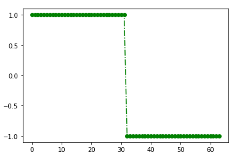
Generally, we use MATLAB or SCIPY's FFT [8] algorithm for signal spectrum analysis. But in fact, FFT is only suitable for signals with limited harmonic frequencies; and the harmonics of sinusoidal DA-fitted signals are infinite, so it is not suitable to analyze this signal with FFT. Typically such as a 2-point DA sine fitting signal:
(1)
[TeX:] $$f(t)=\left[u(t)-u\left(t-\frac{1}{2} T\right)\right]-\left[u\left(t-\frac{1}{2} T\right)-u(t-T)\right].$$According to Fourier decomposition theory, the Fourier series of this signal is as follows:
(2)
[TeX:] $$f(t)=\frac{4}{\pi}\left[\sin \left(\omega_1 t\right)+\frac{1}{3} \sin \left(3 \omega_1 t\right)+\frac{1}{5} \sin \left(3 \omega_1 t\right)+\cdots\right].$$For the convenience of analysis, we sample the signal at 64 points in a single cycle, and call Python's built-in FFT algorithm for analysis. Before FFT analysis, we need to generate a 64-point sampling sequence of the signal. The signal image is presented in Fig. 1.
Then we call Python's built-in FFT algorithm to analyze and the output of amplitude and phase angle. Combining the theoretical value of formula (2) and the calculated value obtained by the program, the data is shown in Table 1.
Table 1.
| 1 | 2 | 3 | 4 | 5 | |
|---|---|---|---|---|---|
| FFT | [TeX:] $$0.637 \angle-1.522$$ | - | [TeX:] $$0.213 \angle-1.424$$ | - | [TeX:] $$0.129 \angle-1.325$$ |
| Normalized amplitude | 1 | - | 0.334 | - | 0.203 |
| Theoretical value | 1 | - | 1/3 | - | 1/5 |
| Theoretical error (%) | 0 | - | 0.3 | - | 1.5 |
As can be observed in Table 1, even if the 2-point DA sine fitting signal is sampled at 64 points, the normalized relative error of the 5th harmonic is still 1.5%. Obviously, the built-in FFT algorithm has obvious errors for theoretical analysis. Therefore, it is necessary to re-derive the Fourier series correlation algorithm of the N-point DA sine fitting signal.
3. Theory Derivation and Algorithm Description
For the N-point DA sequence, the signal is obtained by uniformly sampling a sinusoidal signal with a period of T1. Since at each sampling interval, the signal can be expressed as the multiplication of the sampled value and the unit pulse signal, the N-point DA sequence can be expressed as
According to the definition of Fourier series, its Fourier series expansion expression is:
(4)
[TeX:] $$F(t)=\sum_{n=1}^{\infty} a_n \cos \left(n \omega_1 t\right)+b_n \sin \left(n \omega_1 t\right).$$Its DC component is:
(5)
[TeX:] $$a_0=\frac{1}{T_1} \int_0^{T_1} f(t) d t=\frac{1}{T_1} \sum_0^{N-1} f[i] \frac{T_1}{N}=\frac{1}{N} \sum_0^{N-1} f[i].$$For the magnitude of the cosine component, there are:
For the magnitude of the sine component, there are:
Obviously, for the general term of (3),
Putting (8) into (6), we can get:
In it
Putting (10) into (9), we can get:
(11)
[TeX:] $$a[n]_i=\frac{1}{n \pi} f[i]\left[\sin \frac{2 n \pi}{N}(i+1)-\sin \frac{2 n \pi}{N}(i)\right] .$$Putting (3) into (5), and according to (9), the amplitude of the cosine component of the DA sequence can be obtained as:
(12)
[TeX:] $$a[n]=\sum_0^{N-1} a[n]_i=\frac{1}{n \pi} \sum_0^{N-1} f[i]\left[\sin \frac{2 n \pi}{N}(i+1)-\sin \frac{2 n \pi}{N}(i)\right].$$Similarly, the amplitude of the sine component of the DA sequence is:
4. Experimental Results
4.1 The 2-, 3-, 4-Point Sine Fitting Signals Harmonic Analysis
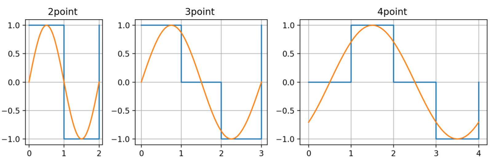
Consider that when the number of points is small, it is easy to formulate the Fourier series of the corresponding signal. So the formula analysis method is used here. Obviously, ignoring the influence of the initial phase of the system, when we approximate the sine wave with 2, 3, and 4 points, it can always be attributed to the following three waveforms (the horizontal axis unit 1 is the minimum DA output time of the system). The three signal diagrams are shown in Fig. 2.
For a 3-point sinusoidal fit signal, we bring the value 3 into formulas (12) and (13), the cosine component coefficient is 0, and the sinusoidal component coefficient is:
According to formulas (4) and (14), the 3-point DA sinusoidal fitting signal can be expressed as:
(15)
[TeX:] $$f(t)=\frac{3 E}{2 \pi}\left[\sin \left(\omega_1 t\right)+\frac{1}{2} \sin \left(2 \omega_1 t\right)+\frac{1}{4} \sin \left(4 \omega_1 t\right)+\frac{1}{5} \sin \left(5 \omega_1 t\right)+\cdots\right].$$For the 4-point DA sine fitting signal, the same can be obtained:
(16)
[TeX:] $$\begin{gathered} f(t)=\frac{E}{\pi}\left[\sin \left(\omega_1 t\right)+\frac{1}{3} \sin \left(3 \omega_1 t\right)+\frac{1}{5} \sin \left(5 \omega_1 t\right)+\cdots\right]+\frac{E}{\pi}\left[-\cos \left(\omega_1 t\right)+\right. \\ \left.\frac{1}{3} \cos \left(3 \omega_1 t\right)-\frac{1}{5} \cos \left(5 \omega_1 t\right)+\cdots\right] . \end{gathered}$$Based on the Fourier series of the above three signals, i.e., formulas (2), (15), (16), the analysis data is shown in Table 2. T0 is the shortest digital-to-analog conversion (DAC) time, total harmonic distortion (THD) is obtained from the Euler natural number square sum formula, which is limited by space and will not be deduced.
Table 2.
| Fundamental wave | Nearest harmonic | Nearest normalized amplitude | THD | |
|---|---|---|---|---|
| 2 points | [TeX:] $$f 0=\frac{1}{2 \mathrm{T}_0}$$ | [TeX:] $$3 f 0=\frac{3}{2 \mathrm{T}_0}$$ | [TeX:] $$\frac{1}{3}$$ | 0.483 |
| 3 points | [TeX:] $$f 0=\frac{1}{3 \mathrm{T}_0}$$ | [TeX:] $$2 f 0=\frac{2}{3 \mathrm{T}_0}$$ | [TeX:] $$\frac{1}{2}$$ | 0.6798 |
| 4 points | [TeX:] $$f 0=\frac{1}{4 \mathrm{T}_0}$$ | [TeX:] $$3 f 0=\frac{3}{4 \mathrm{T}_0}$$ | [TeX:] $$\frac{1}{3}$$ | 0.483 |
As can be seen from Table 2, at the highest frequency of the signal, 3-point and 4-point signals have no advantage over 2-point signals. That is, when the DDS frequency is increased to 4 points or less, it is better to use the 2-point signal directly.
4.2 Harmonic Analysis of Sine Fitting Signal with 5 Points and above
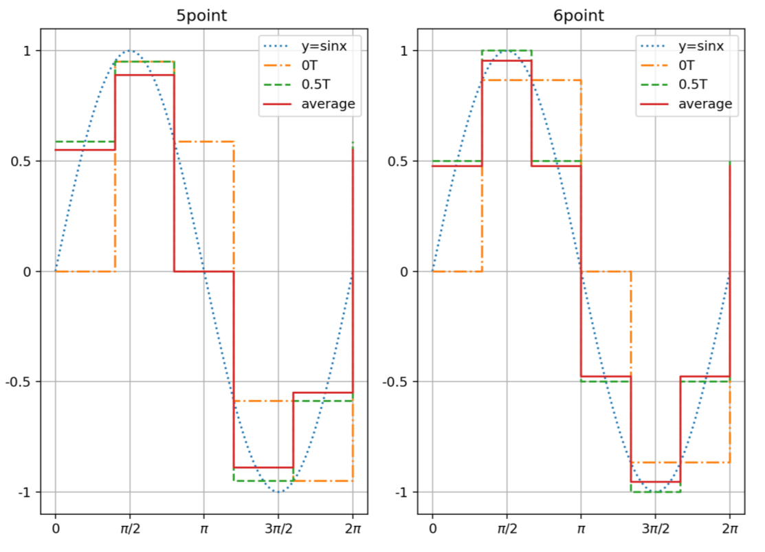
When using DA to fit a sine wave, the conventional method is to use the value at time 0 to represent the value of the time period [0, 1]. Considering that 0.5 moment and [0, 1] integral average of the time period are also two very competitive methods. The three methods will be compared and analyzed. The time-domain diagrams of the three sampling methods of the 5- and 6-point sine fitting signal are shown in Fig. 3.
For sampling at time 0, the sequence is shown in Fig. 3 at the label “0T.” For sampling at the midpoint, it is necessary to offset the sampling time at the original 0 time by 0.5T; the sequence is shown in Fig. 3 at the label “0.5T.” The sampling of the integral average value is mainly obtained by the method of the original function; the sequence is shown in Fig. 3 at the label “average.”
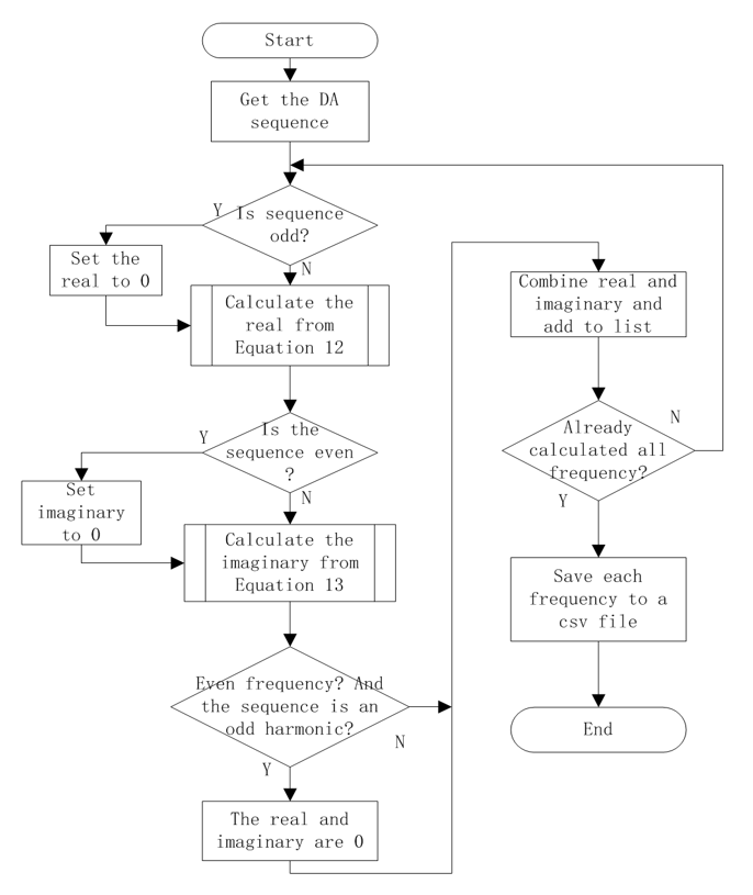
After the DA fitting sine wave is obtained, the theoretical analysis work can be completed by using the above formulas (4), (5), (12), and (13). Its data generation flow chart is presented in Fig. 4.
By using the derived formula to analyze the above three sampling methods, it is found that their harmonic normalized amplitude values are all the same; the phase angle of the middle moment and of the integral average is fixed as π/2. The harmonic analysis values of 5- and 6-point sine fitting (in order to facilitate the discovery of the law, the algorithm is not divided by π) are shown in Table 3.
Table 3.
| Harmonic | 5-point sine fitting signal | 6-point sine fitting signal | ||||||
|---|---|---|---|---|---|---|---|---|
| Modulus | Normalized modulus | Phase angle | Fractional phase angle | Fractional phase angle | Normalized modulus | Phase angle | Fractional phase angle | |
| 1 | 2.9389 | 1.0000 | 2.1991 | π7/10 | 3 | 1.0000 | 2.0944 | π8/12 |
| 2 | 0 | 0 | - | - | 0 | 0 | - | - |
| 3 | 0 | 0 | - | - | 0 | 0 | - | - |
| 4 | 0.7347 | 0.2500 | 0.9425 | π3/10 | 0 | 0 | - | - |
| 5 | 0 | 0 | - | - | 0.6 | 0.2000 | 1.0472 | π4/12 |
| 6 | 0.4898 | 0.1667 | 2.1991 | π7/10 | 0 | 0 | - | - |
| 7 | 0 | 0 | - | - | 0.4286 | 0.1429 | 2.0944 | π8/12 |
As shown in Fig. 3, in the comparison of the harmonic non-normalized amplitude of the three sampling methods, time 0 and time 0.5 are the same, which is greater than the harmonic amplitude of the integral median. In the 5–32 point sampling performed by the author, the rules of the three sampling methods are fixed and there is no change.
Analysis 5–32 points (limited to space, not listed here), and find that the follow-up law is the same as the harmonic law of the 5- and 6-point sine fitting signals. For N-point sine DA fitting signal, the main rules are as following:
1) Non-zero harmonics:
2) The normalized harmonic amplitude is:
3) Corresponding to KN+1 and KN+N-1 harmonics, the phase angle is fixed as:
As shown in Eqs. (17)–(19), for the sampling methods at time 0.5 and integral median, their non-zero harmonics and normalized harmonic amplitudes are the same as at time 0.Their phase angle is fixed at π/2 (i.e., only the sine component).
4.3 Conclusion Test and Practical Value
Through the above analysis, it can be seen that the 0.5 time and the median integral method are completely equivalent. Compared with the traditional sampling at time 0, they have no advantage in filtering. However, it is even doubtful whether there is a better method for sampling at equal intervals. For uniform sampling, the harmonics that need to be filtered start at [TeX:] $$(N-{1})^*f_1,$$ and the normalized amplitude is 1/(N–1). This conclusion is of great significance to the filter design behind DDS. That is, if only the fundamental wave is retained, the cut-off frequency of the filter should be located at [TeX:] $$(\mathrm{N}-1) f_1$$, and the harmonic attenuation is the product of the filter attenuation and 1/(N–1).
In Table 1, through the formula of Fourier series and FFT data, we find that the error of analyzing DDS spectrum with FFT is too large. But there is no doubt that FFT is still the simplest test method for the new formula derived in this paper. Combined with Table 3 and FFT, the data comparison of 5-point sine fitting signal is as follows:
(*1) For the 0.5T, the method phase angle in the paper is fixed at 1.5708;
(*2) For the integral, the method phase angle in the paper is fixed at 1.5708.
It can be seen from Table 4 that after 64 points (worse if less than 64 points) are extended for each state of 5-point sine fitting signal, the non-zero harmonics, amplitude and phase are similar to those derived in this paper, but obviously the FFT data has poor fractional characteristics and sequence rules.
Table 4.
| Harmonic | Modulus | FFT 0T | FFT 0.5T | FFT integral | Phase | FFT-0T phase | FFT-0.5 phase *1 | FFT-integral phase *2 |
|---|---|---|---|---|---|---|---|---|
| 1 | 1.0000 | 1.000 | 1.000 | 1 | 2.1991 | 2.1893 | 1.5610 | 1.5610 |
| 2 | 0 | 0 | 0 | 0 | - | - | - | - |
| 3 | 0 | 0 | 0 | 0 | - | - | - | - |
| 4 | 0.2500 | 0.2411 | 0.2499 | 0.2498 | 0.9425 | 0.9032 | 1.5315 | 1.5315 |
| 5 | 0 | 0 | 0 | 0 | - | - | - | - |
| 6 | 0.1667 | 0.1724 | 0.1666 | 0.1664 | 2.1991 | 2.1402 | 1.5119 | 1.5319 |
| 7 | 0 | 0 | 0 | 0 | - | - | - | - |
| 8 | 0 | 0 | 0 | 0 | - | - | - | - |
| 9 | 0.1111 | 0.1029 | 0.1108 | 0.1108 | 0.9425 | 0.8451 | 1.4824 | 1.4584 |
4.4 Calculation Errors and Processing
In the environment studied by the author, the Python version is 3.9.1, 64bit. However, due to the finite word length effect, there are still obvious calculation errors in the calculation. Considering the common calculation method error handling principles [8], the main error elimination methods used are as follows:
1) For f[n], if the absolute value difference between f[i] and the previous value is less than 10–8, let f[i] equal the previous value.
2) For f[n], if the absolute value difference between f[i] and 0 is less than 10–8, then f[i] equal 0;
3) Judge whether f[n] is an odd function, even function, or odd harmonic function. If it is, clear the corresponding cosine component, sine component, and even harmonic to 0.
5. Conclusion and Open Issues
In this paper, through formula derivation and calculation simulation, the relevant formulas and algorithms of the Fourier series of the N-point DA sine fitting signal are obtained. Through data analysis, the question that sampling at the intermediate time and sampling at the integral average value is better than sampling at time 0 is eliminated. The fractional form of harmonic amplitude and phase angle is given depending on the numerical value. However, due to the limited level of the author, no theoretical proof has been given for the above-mentioned fractional form.


References
- 1 I. V . Ryabov, S. V . Tolmachev, and D. A. Chernov, "A direct digital synthesizer of compound wideband signals," Instruments and Experimental Techniques, vol. 57, pp. 420-425, 2014.doi:[[[10.1134/s0020441214040095]]]
- 2 C. Liu, R. Xu, and Z. Chen, "The systematic analysis of the spectrum structure of DDS signal," Journal of National University of Defense Technology, vol. 27, no. 6, pp. 53-56, 2005.doi:[[[10.3969/j.issn.1001-2486.2005.06.012]]]
- 3 C. E. Calosso, A. C. C. Olaya, and E. Rubiola, "Phase-noise and amplitude-noise measurement of DACs and DDSs," IEEE Transactions on Ultrasonics, Ferroelectrics, and Frequency Control, vol. 67, no. 2, pp. 431439, 2020.doi:[[[10.1109/fcs.2019.8856100]]]
- 4 D. Fu, "Analysis and simulation of DDS stray," Shipboard Electronic Countermeasure, vol. 41, no. 1, pp. 9093, 2018custom:[[[-]]]
- 5 Y . F. Kroupa, "Spectral properties of DDFS: computer simulations and experimental verifications," in Proceedings of IEEE 48th Annual Symposium on Frequency Control, Boston, MA, 1994, pp. 613-623.doi:[[[10.1109/freq.1994.398272]]]
- 6 S. Nikseresht and S. J. Azhari, "A new current-mode computational analog block free from the body-effect," Integration, vol. 65, pp. 18-31, 2019.doi:[[[10.1016/j.vlsi.2018.10.008]]]
- 7 B. Xiao, D. Fan, W. Wang, and Y . Liu, "Development of a high-precision phase micro stepper 1 PPS signal generator," Journal of Time and Frequency, vol. 10, no. 4, pp. 275-283, 2019.custom:[[[-]]]
- 8 E. Bezzam, S. Kashani, P . Hurley, and M. Simeoni, "pyFFS: a Python library for fast fourier series computation," 2022 (Online). Available: https://arxiv.org/abs/2110.00262.custom:[[[https://arxiv.org/abs/2110.00262]]]