Si-Ung Kim and Nammee Moon
Improvement of Object Classification Performance Using a Fusion Optimizer
Abstract: Training deep learning models involves the use of various optimization algorithms, each with its own advantages and disadvantages. Stochastic gradient descent (SGD) provides consistent performance and stable optimization but has the drawback of a slow convergence rate. On the other hand, Adam offers the advantage of fast convergence but can lead to overfitting. This study proposes a hybrid method that combines the stable convergence of SGD with the fast convergence of Adam, enabling the model to be optimized quickly and stably. This approach was applied to the EfficientNetV2 and Vision Transformer (ViT) architectures in image classification tasks. EfficientNetV2 used Adam up to the 6th block and then switched to SGD, achieving the best performance on the proposed dataset with an accuracy of 97.84%, a loss of 0.0990, and an F1-score of 98.04%. Similarly, ViT used Adam for the first 10 encoders and then switched to SGD for the remaining 10 encoders, showing optimal results on the same dataset with an accuracy of 98.54%, a loss of 0.1345, and an F1-score of 98.53%. This fusion optimizer approach effectively enhances training by using Adam for initial feature extraction and SGD for later stages.
Keywords: Convolution Neural Network , Image Classification , Optimizer Fusion , Vision Transformer
1. Introduction
Image classification in computer vision involves classifying images into predefined classes through artificial intelligence training. This classification is primarily performed using two main architectures namely the convolution neural network (CNN) and Vision Transformer (ViT). Both architectures extract features from images to perform classification. CNN are composed of multiple layers, with each layer playing a role in extracting features from the input data. In this context, the initial layers learn simple patterns such as edges and corners, which represent local features. Subsequently, these features are used by deeper layers to learn more complex patterns and abstract features [1]. One of the advantages of CNNs is their ability to effectively extract and combine local features. However, local feature extraction leads to inherent spatial hierarchies and induced biases, which can result in poor performance on small datasets [2]. Meanwhile, ViT effectively considers global information, such as the average brightness and color of an image, by dividing the image into multiple patches and processing them through a self-attention mechanism, delivering effective performance even on small datasets. However, owing to its structural characteristics, it requires more memory and incurs higher computational cost than CNN, and its performance can deteriorate if the image size is too small [2]. Due to variations in performance caused by data size or characteristics, it is not possible to generalize which architectural approach performs best. Additionally, in deep learning, an optimizer is an algorithm used to adjust the weights of a neural network during training to minimize the loss function, and it optimizes learning by iteratively updating the model parameters based on computed gradients.
In this study, we propose a method that applies different optimization techniques to each layer of the image processing architecture, tailored to low-level and high-level feature learning in image learning structures using two different architectures. The layers that extract low-level features require relatively less computational power and can be trained quickly. In contrast, the layers that extract high-level features demand more computational resources, enabling more stable and generalized learning. This differentiated optimization approach is expected to significantly enhance learning efficiency compared to traditional methods using a single optimizer.
Section 2 in this study, describes related research on CNN and ViT architectures. Section 3 describes the optimizer fusion algorithms and the experimental setup and experimental results. Section 4 conclusions based on those results.
2. Related Works
2.1 Image Classification
Recent studies have conducted experiments comparing the performance of CNN and ViT. The paper authored by Gai et al. [3] focused on lung cancer identification and adopted sharpness-aware minimization to control model weights by considering the loss function landscape. Their results reported that EfficientNet3D achieved 95.3% accuracy and the small data efficient transformer (DeiT-S) achieved 85.9% accuracy under identical conditions. Additionally, Huang et al. [4] investigated recycling trash classification and found that the ViT model achieved the highest accuracy of 96.98%, while the CNN model using DenseNet169 achieved 95%. However, these findings illustrate that classification performance can vary significantly depending on the dataset and the specific task at hand. This variation implies that it is challenging to generalize which model CNN or ViT performs better overall across all scenarios. The effectiveness of each model depends on various factors, including the nature of the data and the specific requirements of the task.
To demonstrate the effectiveness of the optimizer fusion methodology, we will conduct experiments using CNN and ViT architectures.
2.1.1 EfficientNetV2
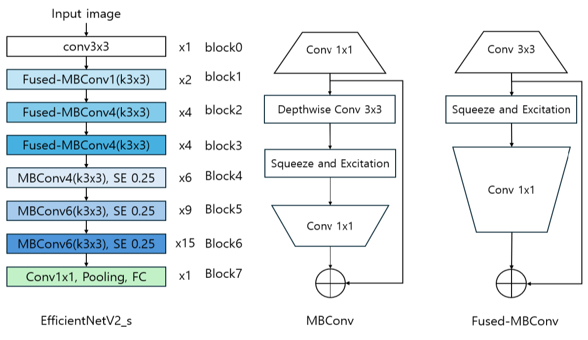
A CNN is a deep learning model used in computer vision. CNN efficiently extracts image features and learning patterns. Among various CNN models, EfficientNetV2, with good performance in various image fields, was used. Fig. 1 shows the structure of EfficientNetV2. EfficientNetV2 is built on two important concepts, MBConv and Fused-MBConv. MBConv is designed to improve computational efficiency through depthwise and pointwise convolutions. In an MBConv block, the process begins with a pointwise convolution Conv 1×1 to expand the number of channels. This is followed by a depthwise convolution Conv 3×3, which applies a separate filter to each channel individually, reducing computational cost. Finally, another pointwise convolution reduces the number of channels back to a smaller size. Some MBConv blocks also include a squeeze-and-excitation (SE) module, which helps the model learn which channels are most important, enhancing overall performance. Fused-MBConv improves upon this by combining the depthwise and pointwise convolutions into a single 3×3 convolution, simplifying the computation and speeding up processing in the earlier layers of the network. Building on these two core concepts, EfficientNetV2 is designed for enhanced efficiency and performance, comprising seven blocks where each processes information as follows:
Block 0 uses a 3×3 convolution to extract low-level features from the image, representing the initial feature extraction phase. Blocks 1 to 3 utilize Fused-MBConv layers. These layers combine the depthwise and pointwise convolutions of traditional MBConv into a single convolution operation to speed up processing. However, using Fused-MBConv across all layers would actually increase parameters and computation, so it is only employed in the initial layers. Blocks 4 to 6 employ MBConv layers, which reduce computational load through depthwise convolution and enhance high-level feature extraction by reducing the number of channels in the SE blocks to 0.25. SE blocks compress global spatial information to learn inter-channel relationships, adjusting the importance of each channel to improve model performance. Block 7 integrates the extracted features using a 1×1 convolution and progresses to classification through a pooling layer and a fully connected layer [5].
2.1.2 Vision Transformer
ViT model is an innovative approach that effectively adapts natural language processing (NLP) techniques for image classification. Similar to how NLP models handle sequences of text, ViT processes images by dividing them into small patches and converting these patches into a sequence. The core idea of this model is to treat each patch of an image as a token, and these patches are then flattened into a one-dimensional sequence that can be processed by the Transformer model Fig. 2.
Specifically, when an image is input into the model, it is first divided into fixed-size patches. Since each patch is a two-dimensional array, it is flattened into a one-dimensional vector and then mapped into an embedding space. To address the potential issue of losing spatial information due to simple patch ordering, positional encoding is added to each patch. This positional encoding allows the Transformer model to understand the order and relative positions of the patches.
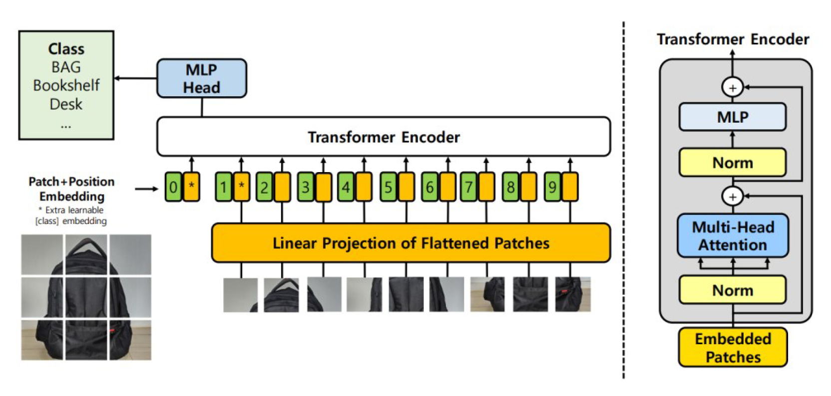
The embedded patch sequence is then passed through multiple layers of Transformer encoders. Each Transformer encoder layer learns how a given patch interacts with other patches in the image, a process driven by the self-attention mechanism.
The first step in a Transformer encoder is to apply layer normalization to the input patch embeddings. This normalization helps the model handle variations in the distribution of input data more effectively. After normalization, the embeddings are projected into Queries, Keys, and Values using three weight matrices, Wq, Wk, and Wv, respectively. The Query acts like a "question" about a particular patch, exploring its relationships with other patches. The Key summarizes important features of each patch, while the Value carries the actual information about the patch.
In the self-attention mechanism, the dot product between the Query and Key is computed to measure the similarity between patches. This similarity score indicates how much attention should be given to a particular patch in relation to others. These attention scores are then normalized using the softmax function, which assigns a relative importance to each patch. The normalized attention scores are used to compute a weighted sum of the Values, generating a new output vector that reflects the most relevant patches.
As this process is repeated across multiple layers of Transformer encoders, the model learns to capture global relationships and contextual information between distant patches in the image. ViT learns the interactions between patches across the entire image, allowing it to better understand the overall structure and patterns within the image [2].
2.2 Optimizer Fusion
Research on optimizer fusion involves using Adam and stochastic gradient descent (SGD) simultaneously to leverage the advantages of each optimizer during training. Each mini-batch utilizes both Adam and SGD to calculate their respective contributions and update the model parameters accordingly [6]. However, calculating and reflecting the contributions of both optimizers leads to slower training speeds compared to using a single optimizer. To enhance the efficiency of deep learning, forward fusion combines forward computation and optimizer updates to delay parameter updates, thus improving data access efficiency. Conversely, backward fusion combines gradient computation and optimizer updates to expedite parameter updates, increasing parallelism and reducing memory access time [7]. However, these methods do not require global information, which can limit their effectiveness with specific optimizers like Adam or root mean square propagation (RMSprop). There is a study that improves performance by using Adam at the beginning of the model and then switching the optimizer to SGD based on certain conditions [8]. This study is very similar to the methodology we propose. However, a key difference from our research is that the process of switching from Adam to SGD occurs only once throughout the entire training process of the model.
In this study, we will experiment with using various optimizers such as SGD, Adam, AdamW, RAdam, and NAdam to learn low-level features in the early layers and high-level features in the deeper layers, by fusing optimizers layer by layer. We aim to find the optimal combination of optimizers to enhance model performance, comparing this method across two different architectures.
3. Methods
3.1 Optimizer Fusion Algorithm
In deep learning, the method of feature extraction from images involves a hierarchical transformation from low-level features, such as edges and textures, to high-level, abstract features like objects and patterns. This enables the first layer to extract simple characteristics at the pixel level of the raw image, while subsequent layers extract more abstract and meaningful features.
The SGD updates weights based on gradients for stable training. Because the model is trained, SGD uses the gradient to adjust the weights, thereby conducting stable training [9].
The Adam optimizer combines momentum and RMSprop algorithms, dynamically adjusting the learning of each parameter to achieve faster and more effective model training. It estimates biased first and second moments, denoted as [TeX:] $$m_{t+1} \text { and } v_{t+1}$$ respectively, for each parameter. Additionally, it corrects the bias in moment estimates using [TeX:] $$b_{t+1},$$ and updates parameters using the corrected estimates [10].
(2)
[TeX:] $$\begin{gathered} m_0=0, v_0=0 \\ m_{t+1}=\beta_1 m_t+\left(1-\beta_1\right) \nabla \mathrm{J}\left(\theta_t\right) \\ v_{t+1}=\beta_2 v_t+\left(1-\beta_2\right) \nabla \mathrm{J}\left(\theta_t\right)^2 \\ \widehat{m}_{t+1}=\frac{m_{t+1}}{1-\beta_1^{t+1}} \\ \widehat{v}_{t+1}=\frac{v_{t+1}}{1-\beta_2^{t+1}} \\ \theta_{t+1}=\theta_t-\eta_t \frac{\widehat{m}_{t+1}}{\sqrt{\widehat{v}_{t+1}}+\epsilon} \end{gathered}$$Through this combination, the Adam optimizer enables rapid convergence in the initial training phases. This initial rapid convergence helps in efficiently navigating the complex loss landscape and reducing training time. We utilize two different optimizers for layers extracting low-level and high-level features, respectively, leveraging the strengths of each during training.
The parameter values learned by Adam up to the low-level layer i can be denoted as [TeX:] $$\theta_t^i .$$ After reaching the high-level layer j, which extracts high-level features, the optimizer is switched to SGD to continue the training. In this case, the parameters [TeX:] $$\theta_t^i$$ learned by Adam are used as the initial input for SGD. The mathematical formulation for this training process is as follows:
(3)
[TeX:] $$\begin{gathered} m_t^i=\beta_1 m_{t-1}^i+\left(1-\beta_1\right) \nabla \mathrm{J}\left(\theta_{t-1}^i\right) \\ v_t^i=\beta_2 v_{t-1}^i+\left(1-\beta_2\right)\left(\nabla \mathrm{J}\left(\theta_{t-1}^i\right)\right)^2 \\ \widehat{m}_t^i=\frac{m_t^i}{1-\beta_1^t} \\ \widehat{v}_t^i=\frac{v_t^i}{1-\beta_2^t} \\ \theta_t^i=\theta_{t-1}^i-\eta_{t-1} \frac{\widehat{m}_t^i}{\sqrt{\widehat{v}_t^i}+\epsilon} \\ \theta_{t+1}^j=\theta_t^i-\eta_t \nabla \mathrm{~J}\left(\theta_t^j\right) \end{gathered}$$3.2 Experimental Setup
The dataset comprises various object data collected through crowd sourcing, including images gathered from diverse environments such as web crawling, cameras, and smartphone photography. To minimize class imbalance and ensure model stability, the dataset includes more than 600 images per class across 18 classes, including items such as bags, golf bags, blankets, bicycles, bookshelves, and chairs. Additionally, the CIFAR-10 dataset, consisting of 10 classes with 6,000 images per class, totaling 60,000 images evenly distributed among the classes, was used. A summary of the data instances for each category in the proposed dataset is provided in Table 1.
Table 1.
| Class | Count | Class | Count |
|---|---|---|---|
| Bookshelf | 727 | Display stand | 819 |
| Chair | 1,411 | Refrigerator | 646 |
| Chair wheels | 1,578 | Flowerpot | 965 |
| Frame | 1,382 | Toy | 1,863 |
| Partition | 939 | Marble table | 698 |
| Bag | 1,740 | Hanger | 730 |
| Golf bag | 938 | Desk | 761 |
| Bedding | 1,056 | Wardrobe | 910 |
| Sofa | 1,047 | Bicycle | 1,658 |
We conducted an experimental comparison between CNN and ViT models using the EfficientNetV2 model, which was pretrained on ImageNet, as the CNN basis. For the ViT model, we utilized the ViT-B/16, also pretrained on the same dataset. Across the experiments, we maintained consistent settings for image size 244×244. A batch size of 128 was used to balance memory usage and computational efficiency. The experiments were run for 10 epochs to provide sufficient training time for the models to converge. For the loss function, we employed cross entropy, which is widely used in classification tasks due to its effectiveness in handling multi-class problems. To ensure a fair comparison, we kept all these settings constant and only varied the optimizer. These experiments were carried out on a Windows 10 platform equipped with an Intel Core i7 8700K processor and an NVIDIA RTX 4090 graphics card, using PyTorch 2.2.2.
The model was evaluated based on accuracy and the F1-score, which is the harmonic mean of precision and recall. Accuracy represents the proportion of correct classifications by the model. The F1-score is a performance metric derived from precision and recall, where precision indicates how accurately the model identifies true positives out of all positive predictions, and recall implies how well the model identifies true positives out of the actual positives. This method is robust against imbalanced class distribution in the model and is a useful indicator of overall performance.
(4)
[TeX:] $$F 1-\text { score }=2 \times \frac{\text { Precision } \times \text { Recall }}{\text { Precision }+ \text { Recall }}$$The only variable changed between experiments was the optimizer, ensuring that differences in performance can be attributed solely to the optimization strategy.
3.3 Experimental Results
During training, to apply two different optimizers for each layer, we defined the section trained with the first optimizer as the low-level layer and the section trained with the second optimizer as the high-level layer. Training was conducted based on this definition.
The Experiment 1 results obtained with different optimizers for training are summarized in Table 2. In the experiments, using the EfficientNetV2 model on the proposed dataset, applying Adam for feature extraction up to the 6th block and SGD for the remaining blocks yielded the highest results with an accuracy of 97.89%, a loss of 0.0990, and an F1-score of 98.04%. For the CIFAR-10 Dataset, using Adam up to the 6th block and SGD thereafter achieved the best performance with an accuracy of 93.74%, a loss of 0.2311, and an F1-score of 93.71%. When training the ViT model on the proposed dataset, using Adam for the first 10 Transformer encoders and SGD for the subsequent encoders resulted in the highest metrics with an accuracy of 97.84%, a loss of 0.1345, and an F1-score of 97.85%. Similarly, for the CIFAR-10 dataset, using Adam up to the 10th Transformer encoder and SGD for the remaining encoders produced the best results with an accuracy of 94.75%, a loss of 0.1833, and an F1-score of 94.69%.
Through this, the first experiment confirmed that for both deep learning models operating in different ways, using Adam's rapid convergence for early low-level feature extraction in low-level layers and then updating the parameters with SGD in high-level layers, which provides consistent performance and stability for deep high-level feature extraction, resulted in higher performance.
In the second experiment, we investigated whether using various variants of Adam could lead to faster convergence or higher performance compared to the standard Adam optimizer. The optimizers used in this experiment included AdamW, which enhances generalization performance by applying weight decay to the original Adam, RAdam, which reduces the instability of early training in Adam, and NAdam, which achieves faster convergence than Adam. In this experiment, we applied Adam and its variants in the low-level layers for early feature extraction and used SGD in the high-level layers for later stages of training. This setup allowed us to determine which optimizer achieves the best convergence in the low-level layers.
The Experiment 2 results obtained with different optimizers for training are summarized in Table 3. The fusion optimizer using the Adam optimizer demonstrated the highest performance across all datasets for both the EfficientNetV2 and ViT models. Specifically, for the EfficientNetV2 model, using the Adam optimizer on the proposed dataset resulted in an accuracy of 97.89%, a loss of 0.0990, and an F1-score of 98.04%. On the CIFAR-10 dataset, it achieved an accuracy of 93.74%, a loss of 0.2311, and an F1-score of 93.71%. For the ViT model, the Adam optimizer on the proposed dataset achieved an accuracy of 97.74%, a loss of 0.0945, and an F1-score of 97.48%, while on the CIFAR-10 dataset, it resulted in an accuracy of 94.75%, a loss of 0.1833, and an F1-score of 94.69%. These findings indicate that the fusion of Adam with other optimizers, particularly in combination with SGD, produced the best performance.
Table 2.
| Model | Dataset | Low-level layer optimizer | Layer set to low-level | High-level layer optimizer | Accuracy (%) | Loss | F1-score (%) |
|---|---|---|---|---|---|---|---|
| EfficientNetV2 | proposed | SGD | All block | - | 97.20 | 0.1534 | 97.42 |
| Block 0–1 | Adam | 97.69 | 0.1053 | 97.73 | |||
| Block 0–2 | 97.79 | 0.1147 | 97.76 | ||||
| Block 0–3 | 97.74 | 0.1062 | 97.73 | ||||
| Block 0–4 | 97.69 | 0.1019 | 97.61 | ||||
| Block 0–5 | 96.57 | 0.1560 | 96.23 | ||||
| Block 0–6 | 96.52 | 0.1532 | 96.21 | ||||
| Adam | All block | - | 97.03 | 0.1446 | 97.30 | ||
| Block 0–1 | SGD | 95.54 | 0.1986 | 95.01 | |||
| Block 0–2 | 95.59 | 0.2120 | 95.06 | ||||
| Block 0–3 | 95.64 | 0.1658 | 95.12 | ||||
| Block 0–4 | 97.01 | 0.1658 | 96.93 | ||||
| Block 0–5 | 97.84 | 0.1288 | 97.66 | ||||
| Block 0–6 | 97.89 | 0.0990 | 98.04 | ||||
| CIFAR-10 | SGD | All block | - | 91.03 | 0.2665 | 90.83 | |
| Block 0–1 | Adam | 90.11 | 0.3199 | 89.75 | |||
| Block 0–2 | 91.28 | 0.3044 | 91.02 | ||||
| Block 0–3 | 90.71 | 0.3189 | 90.45 | ||||
| Block 0–4 | 91.62 | 0.3620 | 91.33 | ||||
| Block 0–5 | 92.01 | 0.3451 | 91.98 | ||||
| Block 0–6 | 91.42 | 0.2843 | 91.52 | ||||
| Adam | All block | - | 93.45 | 0.2020 | 93.34 | ||
| Block 0–1 | SGD | 91.92 | 0.2786 | 91.07 | |||
| Block 0–2 | 91.06 | 0.3064 | 90.66 | ||||
| Block 0–3 | 90.25 | 0.3418 | 89.73 | ||||
| Block 0–4 | 90.17 | 0.3291 | 89.58 | ||||
| Block 0–5 | 93.85 | 0.2399 | 93.44 | ||||
| Block 0–6 | 93.74 | 0.2311 | 93.71 | ||||
| Vision Transformer | proposed | SGD | All encoder | - | 95.71 | 0.1336 | 95.71 |
| Encoder 0 | Adam | 95.77 | 0.1325 | 95.76 | |||
| Encoder 0–5 | 96.12 | 0.1289 | 95.76 | ||||
| Encoder 0–10 | 96.81 | 0.1330 | 96.81 | ||||
| Adam | All encoder | - | 96.23 | 0.1324 | 96.11 | ||
| Encoder 0 | SGD | 97.07 | 0.1510 | 96.07 | |||
| Encoder 0–5 | 97.51 | 0.1435 | 97.44 | ||||
| Encoder 0–10 | 97.84 | 0.1345 | 97.85 | ||||
| CIAFR-10 | SGD | All encoder | - | 88.05 | 0.3486 | 87.51 | |
| Encoder 0 | Adam | 91.78 | 0.2693 | 91.76 | |||
| Encoder 0–5 | 92.54 | 0.2336 | 92.50 | ||||
| Encoder 0–10 | 92.78 | 0.1770 | 92.78 | ||||
| Adam | All encoder | - | 88.26 | 0.3541 | 87.93 | ||
| Encoder 0 | SGD | 91.04 | 0.2133 | 91.04 | |||
| Encoder 0–5 | 92.13 | 0.2061 | 92.14 | ||||
| Encoder 0–10 | 94.75 | 0.1833 | 94.69 |
Values in bold indicate the best performance achieved during testing.
Table 3.
| Model | Dataset | Low-level layer optimizer | Layer set to low-level | Accuracy (%) | Loss | F1-score (%) |
|---|---|---|---|---|---|---|
| EfficientNetV2 | proposed | Adam | Block 0–6 | 97.89±0.14 | 0.0990±0.010 | 98.04±0.30 |
| AdamW | 97.84±0.05 | 0.1046±0.012 | 97.55±0.33 | |||
| RAdam | 96.91±0.18 | 0.1338±0.040 | 97.32±0.21 | |||
| NAdam | 97.59±0.30 | 0.1800±0.080 | 97.08±0.20 | |||
| CIFAR-10 | Adam | 93.74±0.10 | 0.2311±0.004 | 93.71±0.11 | ||
| AdamW | 93.41±0.14 | 0.2395±0.002 | 93.48±0.20 | |||
| RAdam | 93.41±0.40 | 0.2476±0.023 | 93.45±0.19 | |||
| NAdam | 92.57±0.08 | 0.2715±0.090 | 92.49±0.09 | |||
| Vision Transformer | proposed | Adam | Encoder 0–10 | 97.74±0.04 | 0.0945±0.005 | 97.48±0.03 |
| AdamW | 97.60±0.15 | 0.1093±0.110 | 97.35±0.22 | |||
| RAdam | 97.35±0.15 | 0.1030±0.060 | 97.05±0.25 | |||
| NAdam | 97.35±0.05 | 0.1047±0.040 | 97.16±0.07 | |||
| CIFAR-10 | Adam | 94.75±0.11 | 0.1833±0.007 | 94.69±0.07 | ||
| AdamW | 94.56±0.12 | 0.1755±0.025 | 94.55±0.04 | |||
| RAdam | 94.68±0.18 | 0.1812±0.049 | 94.61±0.024 | |||
| NAdam | 94.43±0.10 | 0.1902±0.050 | 94.44±0.15 |
Values in bold indicate the best performance achieved during testing.
4. Conclusion
This research aims to improve the performance of image classification models by optimizing the selection of optimizers. We conducted experiments on two datasets, the proposed dataset with 18 classes and the CIFAR-10 dataset, using two different model architectures, CNN and ViT. The experimental results showed that for both CNN and ViT, applying Adam in the early layers and then switching to SGD in the later layers yielded the highest performance. Using Adam in the initial stages allows for rapid and effective learning of low-level features, while applying SGD in the later stages ensures consistent and stable learning of high-level features, thereby enhancing the overall model performance. Additionally, we compared various variants of Adam, including AdamW, RAdam, and NAdam, and found that the fusion method using Adam achieved the highest performance.
These experiments confirm that our fusion method is effective in improving performance and can be applied to various architectures, not just specific ones. Future experiments will compare the effectiveness of this method not only on image data but also on other types of data such as audio, time series, and text data, as well as on multimodal data, to further validate its performance.
Biography
Si-Ung Kim
https://orcid.org/0009-0007-2541-5412
He received the B.S. degrees in Computer Science and Engineering from Hoseo University, in 2023 B.S. Kim joined the Department of computer science at Hoseo University, Asan, Korea in 2023. He is currently a Master in the Department of computer science, Hoseo University. He is interested in computer vision, object detection, image generation.
Biography
Nammee Moon
https://orcid.org/0000-0003-2229-4217
She received B.S., M.S., and Ph.D. degrees from the School of Computer Science and Engineering at Ewha Womans University in 1985, 1987, and 1998, respectively. She served as an assistant professor at Ewha Womans University from 1999 to 2003, a then as a professor of digital media, Graduate School of Seoul Venture Information, from 2003 to 2008. Since 2008, has been a professor of computer information at Hoseo University. Her current research interests include social learning, HCI and user-centric data, and big data processing and analysis.
References
- 1 K. O'shea and R. Nash, "An introduction to convolutional neural networks," 2015 (Online). Available: https://arxiv.org/abs/1511.08458.doi:[[[https://arxiv.org/abs/1511.08458]]]
- 2 A. Dosovitskiy, "An image is worth 16x16 words: Transformers for image recognition at scale," 2020 (Online). Available: https://arxiv.org/abs/2010.11929v1.doi:[[[https://arxiv.org/abs/2010.11929v1]]]
- 3 L. Gai, M. Xing, W. Chen, Y . Zhang, and X. Qiao, "Comparing CNN-based and transformer-based models for identifying lung cancer: which is more effective?," Multimedia Tools and Applications, vol. 83, no. 20, pp. 59253-59269, 2024. https://doi.org/10.1007/s11042-023-17644-4.doi:[[[10.1007/s11042-023-17644-4]]]
- 4 K. Huang, H. Lei, Z. Jiao, and Z. Zhong, "Recycling waste classification using vision transformer on portable device," Sustainability, vol. 13, no. 21, article no. 11572, 2021. https://doi.org/10.3390/su132111572.doi:[[[10.3390/su13572]]]
- 5 M. Tan and Q. Le, "EfficientNetv2: smaller models and faster training," Proceedings of Machine Learning Research, vol. 139, pp. 10096-10106, 2021.custom:[[[-]]]
- 6 N. Landro, I. Gallo, and R. La Grassa, "Mixing Adam and SGD: a combined optimization method," 2020 (Online). Available: https://arxiv.org/abs/2011.08042.doi:[[[https://arxiv.org/abs/2011.08042]]]
- 7 Z. Jiang, J. Gu, M. Liu, K. Zhu, and D. Z. Pan, "Optimizer fusion: efficient training with better locality and parallelism," 2021 (Online). Available: https://arxiv.org/abs/2104.00237.doi:[[[https://arxiv.org/abs/2104.00237]]]
- 8 N. S. Keskar and R. Socher, "Improving generalization performance by switching from Adam to SGD," 2017 (Online). Available: https://arxiv.org/abs/1712.07628.doi:[[[https://arxiv.org/abs/1712.07628]]]
- 9 H. Robbins and S. Monro, "A stochastic approximation method," The Annals of Mathematical Statistics, vol. 22, no. 3, pp. 400-407, 1951. https://doi.org/10.1214/aoms/1177729586.doi:[[[10.1214/aoms/1177729586]]]
- 10 D. P. Kirma and J. Ba, "A method for stochastic optimization," 2014 (Online). Available: https://arxiv.org/abs/1412.6980v1.doi:[[[https://arxiv.org/abs/1412.6980v1]]]