SER Performance Analysis of Generalized κ − µ and η − µ Fading Channels

I. INTRODUCTION

A. Background

THE fifth generation (5G) aims to provide higher data rates and lower latency performances than previous generations of wireless communications, enabling new use cases such as virtual reality, autonomous driving, remote e-health, and more [1]–[4]. In 5G wireless communications, performance analysis is a vital aspect of system design [5]. Especially with closed-form performance expressions such as symbol error rate (SER) and signal-to-interference-plus-noise ratio (SINR), one can estimate the wireless communication system performance before actually deploying it.

In wireless communication systems, multipath propagation, fading and shadowing effects exist, which greatly affect the system performance. Besides, SER and SINR are widely used for the system performance analysis [6], [7]. In literature, while analyzing the system performance, generalized channel models are used to describe different propagation phenomena, such as multipath, shadowing, and large and smallscale fading [8]–[11]. In these generalized channel models, the [TeX:] $$\kappa-\mu$$ and [TeX:] $$\eta-\mu$$ distributions [12], as versatile and generalized channel models, can fit well channel modeling and comprise many special cases of fading models like Rayleigh, Rician (Nakagami-n), one-sided Gaussian, Hoyt (Nakagamiq), etc. [13]–[15]. In addition, the [TeX:] $$\kappa-\mu$$ channel is well-suited for modeling line-of-sight (LOS) components, and the [TeX:] $$\eta-\mu$$ channel is characterized by clusters that lack any dominant or LOS components. Accordingly, they can be used to represent various communication scenarios such as micro/macro cellular, hybrid satellite and terrestrial communications [16]–[18]. Therefore, one can obtain some versatile system performance expressions that can be applied in various wireless communication environments based on the generalized channels, which motives us to develop this work.

B. Related Works and Motivation

In system performance analysis, it is generally hard to obtain a closed-form SER or bit error rate (BER) performance expression due to the involved transcendental functions such as exponential integral functions [19]. In order to tackle this issue, moment generating function (MGF) is introduced, which concerns the Marcum Q-function with the closed-loop integral. For instance, the average bit error probability (ABEP) of the L-branch selection combining (SC) receiver was derived with the help of the MGF function under the disturbance of [TeX:] $$\kappa-\mu$$ distribution [20]. The authors in [21] proposed an MGF-based method for BER and SER in the generalized-K fading channels model. [22] presented the closed-form expression for the average BER for the unmanned aerial vehicles (UAV)-assisted dual-hop free-space optical (FSO) system under the Gamma- Gamma atmospheric turbulence model. In [23], considering a mixed asymmetric dual-hop radio frequency (RF) / FSO transmission system subject to the generalized [TeX:] $$\kappa-\mu$$ and [TeX:] $$\mathcal{M} \text {-distribution, }$$ the average BER expression was provided by utilizing cumulative distribution function (CDF) in terms of the Meijer’s G function.

In [24], by employing the contour integral of the Marcum- Q function and the MGF for signal-to-noise ratio (SNR), the authors calculated the detection probability of a maximum ratio combining (MRC) combined energy detector over Nakagami-m fading channels. The authors in [25] developed the MGF expression for the probability density function (PDF) characterizing [TeX:] $$\alpha-\mu$$ channel model, with the aim of evaluating the BER performance. However, the MGF-based approach is constrained by the system and channel parameters that are usually assumed to be integers, which has narrow application scopes [26]–[28]. Subsequently, [26] introduced a new method for closed-form and asymptotic approaches for SER of Mary quadrature amplitude modulation (M-QAM) signal in Fluctuating Beckman fading channel model, in which they represented the MGF by a factorized power type.

In our previous studies, SER performance of the sparse vector coding-based non-orthogonal multiple access (SVCNOMA) system was addressed with different modulation schemes over Rayleigh channels [29]. Similarly, the authors in [30] analyzed the SER performance of the space-time network coding (STNC) with the help of a unified MGF method. Additionally, the study in [31] provided analytical SER expressions based on the M-ary dual-ring star-shaped QAM modulation, which were then applied to derive SER expressions for frequency non-selective slow fading channels. The authors in [32] derived the closed-form expression for SER in a hybrid satellite-terrestrial relay network (HSTRN) over a shadowed-Rician (SR) distribution. This was achieved using the MGF method combined with Taylor series and binomial expansions. Nevertheless, the SER analysis therein only considers some ideal and special cases. Furthermore, [33] has derived the exact SER expressions of spatial modulation multiple input multiple output (SM MIMO) system over [TeX:] $$\eta-\mu$$ channel, but these expressions involve complex Hypergeometric functions, which are hard to tackle. In [34], the SER expressions over [TeX:] $$\kappa-\mu$$ and [TeX:] $$\eta-\mu$$ channels were obtained, but with lower accuracy.

One can know from the literature that most existing studies investigate the SER performance under some ideal or special channels. Although the closed-form SER expressions in [TeX:] $$\kappa-\mu$$ or [TeX:] $$\eta-\mu$$ fading models are investigated, yet the solutions are mostly with lower accuracies. In order to remedy this, we investigate the SER over the generalized [TeX:] $$\kappa-\mu$$ and [TeX:] $$\eta-\mu$$ fading channels, and aim to give more precise system performance expressions in this article. We can gain insights into its capabilities in characterizing various channel fading models by the obtained SER of such generalized channels [35]–[37]. To this end, we introduce some special conditions in line with prior studies in [38]–[40]. Additionally, the authors in [41], [42] solved the computational complicated issue of exponential integral functions by truncating the infinite series, which is also incorporated here. In the end, when solving definite integrals that contain higher-order trigonometric integrals, we attempt to approximate the integral value using numerical integration based on interpolation [43].

C. Contributions and Organization

The main contributions of this work can be summarized as follows:

· We present simplified closed-form expressions for SER over [TeX:] $$\kappa-\mu$$ and [TeX:] $$\eta-\mu$$ channels, which exhibit arbitrarily small errors upon varying the truncation factor T. Besides, our derived approximate SER expressions are with low computational complexity. Furthermore, leveraging our SER analysis in the generalized fading channels, we have demonstrated its applicability in evaluating the SER performance for some classical fading channels.

· Numerical results indicate that: 1) The optimal selection of T is affected by the parameters of channel fading, but a smaller T usually suffices to achieve precise outcomes. 2) SER performance improves with the increasing values of [TeX:] $$\kappa,\mu \text{ and } \eta.$$ Besides, μ has a more pronounced effect than κ and η. 3) Our approximate SER expressions have superior accuracy compared with the previous expressions.

The rest of this paper is organized as follows: Section II presents the relevant preamble to facilitate understanding of the subsequent sections. In Section III, we provide closedform SER expressions for various modulation schemes under generalized fading channels. Based on the generalized SER analysis, we derive the closed-form SER expressions in some classical fading channels. Additionally, we discuss the comparisons with the previous approaches. Next, Section IV shows the numerical analysis of the theoretical values and simulation results. Finally, this paper is concluded by Section V.

II. PRELIMINARIES

According to [6] and [30], the achievable SER is expressed as [TeX:] $$\mathcal{P}=\mathbb{E}[P({err} \mid \gamma)]=\int_0^{\infty} P({err} \mid \gamma) f(\gamma) d \gamma,$$ in which [TeX:] $$\mathbb{E}(\cdot)$$ is the expectation operation, γ denotes the instantaneous SNR and [TeX:] $$P({err} \mid \gamma)$$ represents the conditional SER depending on the modulation scheme. In practical applications, M-ary phase shift keying (M-PSK) and M-QAM are two widely used modulation schemes, we hereby consider the calculation of SER under these two modulations. The conditional SERs for M-PSK and M-QAM modulations are as follows:

where M denotes the modulation order, [TeX:] $$g_p=\sin ^2(\pi / M),$$ [TeX:] $$g_q=\frac{3}{2(M-1)} \text { and } Q(\cdot)$$ indicates the Gaussian Q-function.

III. SER ANALYSIS FOR GENERALIZED FADING SCENARIOS

A. SER Performance Analysis in [TeX:] $$\kappa-\mu$$ Fading Scenario

The [TeX:] $$\kappa-\mu$$ model is a generalized fading model commonly used in the design, analysis and simulation of wireless communication systems to understand the effect of channel fading on signal propagation and link performance. It contains several special channel models, such as Rician (μ = 1, κ = K), Nakagami-m ([TeX:] $$\mu=m, \kappa \rightarrow 0$$) Rayleigh ([TeX:] $$\mu=1, \kappa \rightarrow 0$$) and one-sided Gaussian ([TeX:] $$\mu=0.5, \kappa \rightarrow 0$$). The parameter κ expresses the ratio of the main component power to the total power of the scattered waves, and the parameter μ indicates the number of multipath clusters [44], [45]. In other words, the parameter κ expresses the severity of the fading, with a smaller value of κ indicating more severe fading and a larger value of κ indicating less severe fading. The parameter μ signifies fading diversity. A smaller value of μ corresponds to greater diversity, leading to reduced fading correlation in the channel. Conversely, a larger value of μ results in increased fading correlation [46]. In this case, PDF of γ can be represented as

in which [TeX:] $$\bar{\gamma}=\mathbb{E}(\gamma), I_v(z)$$ denotes the modified Bessel function [47]. Considering t as the adjustment factor, we can rewrite the Bessel function as

where [TeX:] $$\Gamma(\cdot)$$ means the Gamma Function, i.e., [TeX:] $$\Gamma(z)=(z-1) ! .$$

Lemma 1: In line with the equation [TeX:] $$\mathcal{P}=\mathbb{E}[P( { err } \mid \gamma)]=\int_0^{\infty} P({err} \mid \gamma) f(\gamma) d \gamma,$$ the exact SER expressions for M-PSK and M-QAM modulations over [TeX:] $$\kappa-\mu$$ channel are given by

Proof: See Appendix A.

One can find that the expression is hard to tackle here due to the involved infinite factorial and generalized integral expressions. We thus introduce an approximation with a negligible error margin to address this issue, utilizing the truncation operation in subsequent steps to simplify the calculation.

Specifically, according to Lemma 1, these two expressions have the same infinite term, which is

where [TeX:] $$g \in\left\{g_p, g_q\right\}$$ is the modulation dependent parameter. We find that the infinite term (7) has an approximate upper bound. In this case, it is possible to express the SER using an approximation that significantly reduces the computational complexity.

Lemma 2: The [TeX:] $$\mathcal{P}_{p s k}^{\kappa-\mu}$$ can be approximately expressed by truncating the infinite series to the first T terms, which gives

Here the truncation error is

Proof: See Appendix B.

Based on the insights from Lemma 2, it is observed that the infinite series presented in (5) converges within a limited number of terms. Thus it is better to write in terms of T rather than infinity for ease of presentation. Correspondingly, the [TeX:] $$\mathcal{P}_{Q A M}^{\kappa-\mu}$$ in (6) can also be estimated while truncating the infinite series to its first T elements.

In addition, it is noticed that the integral of the above integrable functions cannot be expressed by elementary functions, we thus use the numerical integration method to further approximate the expression of the (8). Here, the Lagrange interpolation scheme is adopted [43], and the detailed analysis is provided in the subsequent lemma.

Lemma 3: The closed-form expressions of SERs for MPSK and M-QAM modulations over [TeX:] $$\kappa-\mu$$ channel are separately given by

where [TeX:] $$A_0$$ a and b are defined as [TeX:] $$A_0=\frac{\mu^\mu(1+\kappa)^\mu}{\pi e^{\mu \kappa} \bar{\gamma}^\mu},$$ [TeX:] $$a=\frac{\mu^2 \kappa(1+\kappa)}{\bar{\gamma}}, b=\frac{\mu(1+\kappa)}{\bar{\gamma}}.$$ And [TeX:] $$\theta_i=i \frac{M-1}{M N} \pi(i \in[1, N])$$ is represented by [TeX:] $$0\lt\theta_1\lt\theta_2 \cdots\lt\theta_N=\frac{M-1}{M} \pi.$$

in which [TeX:] $$\theta_q=q \frac{2 \pi}{N}, \theta_{q^{\prime}}=q^{\prime} \frac{4 \pi}{N}, q \in[1, N] \text { and } q^{\prime} \in[1, N] \text {. }$$

Proof: See Appendix C.

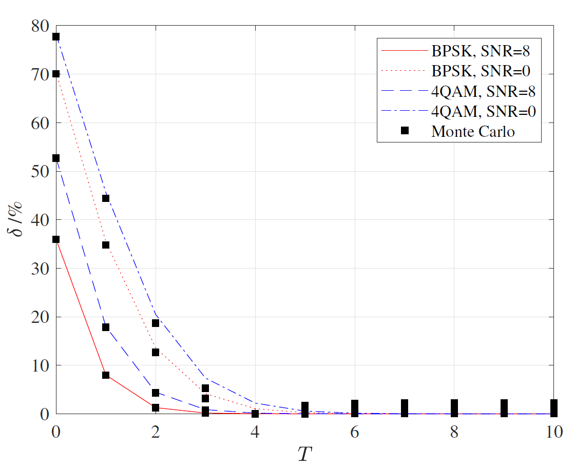
To verify the validity of Lemma 3, we compare these derivations with the exact expressions in [48] and the Monte Carlo (MC) simulation values, and give their relative errors δ in different SNR cases. As shown in Fig. 1, it is noticed that the relative error δ is affected by the truncation parameter T. The truncation T has a great effect on the approximation of SER in low SNR region, when the SNR is higher, this effect becomes weaker. When T is greater than a certain value, the relative error δ tends to be 0, which also verifies the correctness of Lemma 3. Besides, the convergence speed of the relative error δ in the high SNR channel state (SNR = 8) is faster than that in the low SNR channel state (SNR = 0). Our derivation has demonstrated superior performance in terms of accuracy and computational efficiency, making it a more reliable choice for estimating SER under various conditions.

However, when [TeX:] $$\kappa \rightarrow 0,$$ these two expressions do not hold. In what follows, we investigate the SER expressions for this special case. With the estimated expression [TeX:] $$I_{v-1}(z) \approx \frac{(z / 2)^{v-1}}{\Gamma(v)}$$ from [11], (3) will be

When [TeX:] $$\kappa \rightarrow 0,$$ the above formula can be derived as

Therefore, the SER [TeX:] $$\mathcal{P}_{p s k}^{\kappa \rightarrow 0}$$ in the case [TeX:] $$\kappa \rightarrow 0$$ can be given as

Further, according to the relation [TeX:] $$Z=\int_0^{\infty} \gamma^a e^{-b \gamma} d \gamma=\frac{a !}{b^a} \cdot \frac{1}{b}$$ obtained in Appendix A, [TeX:] $$\mathcal{P}_{p s k}^{\kappa \rightarrow 0}$$ is further derived as

Combined with the numerical integration method in Appendix C, we can obtain

Following the same principle, the SER expressions for QAM modulation when [TeX:] $$\kappa \rightarrow 0$$ can also be given as

Remark 1: (i) To further generalize the SER expressions, in addition to (10) and (11), a special case for [TeX:] $$\kappa \rightarrow 0$$ is additionally considered, and the corresponding channel is Nakagamim channel. (ii) For the expressions (10) and (11), we have verified that the approximate SER tends to be stable when the truncation factor T is greater than or equals to a certain value. Following comprehensive experimental validation, we select T = 4 and N = 1000 as the parameters for estimating the SER. This choice balances computational efficiency with high approximation accuracy.

B. SER Performance Analysis in [TeX:] $$\eta - \mu$$ Fading Scenario

The [TeX:] $$\eta - \mu$$ channel model is also a generalized fading model that combines the effects of multipath propagation, interference and shadowing, including Hoyt (μ = 0.5) and Nakagami-m ([TeX:] $$\mu \rightarrow \pm 1$$) and other special cases. The parameter η denotes the shape of the channel fading distribution, and the parameter μ represents the number of multipath clusters or the severity of the fading. It is therefore particularly suitable for characterizing scenarios where both multipath propagation and interference effects are present, such as urban or indoor environments [11], [49]. We have the PDF of γ in [TeX:] $$\eta - \mu$$ channel as

in which [TeX:] $$H^{\prime} \text { and } h^{\prime}$$ are defined as the functions of η. The corresponding PDF in (18) has two formats under the influence of parameters [TeX:] $$h^{\prime} \text { and } H^{\prime}$$, that is, [TeX:] $$h^{\prime}=\frac{2+\eta^{-1}+\eta}{4}$$ and [TeX:] $$H^{\prime}=\frac{\eta^{-1}-\eta}{4}$$ for format 1, whereas, [TeX:] $$h^{\prime}=\frac{1}{1-\eta^2} \text { and } H^{\prime}=\frac{\eta}{1-\eta^2}$$ for format 2. Since the conversion between the two formats is given by a simple bilinear transformation, only format 1 is considered here. By means of the definition of [TeX:] $$I_v(z)$$ in [47], [TeX:] $$I_{\mu-\frac{1}{2}}\left(\frac{2 \mu H^{\prime} \gamma}{\bar{\gamma}}\right)$$ can be expressed as follows:

With the same analysis process under the [TeX:] $$\kappa - \mu$$ channel, we can directly deduce the closed form of SER under the [TeX:] $$\eta - \mu$$ channel, which is given in the following Lemma.

Lemma 4: The achievable SER expressions for M-PSK and M-QAM over [TeX:] $$\eta - \mu$$ channel are represented by (20) and (21), where (21) is given at the bottom of next page.

where [TeX:] $$A_0, a \text { and } b$$ are defined as [TeX:] $$A_0=\frac{2 \sqrt{\pi} \mu^{2 \mu}\left(2+\eta^{-1}+\eta\right)^\mu}{\pi \bar{\gamma}^{2 \mu}(\mu-1) ! 4^\mu},$$ [TeX:] $$a=\frac{\mu\left(\eta^{-1}-\eta\right)}{4 \bar{\gamma}}, b=\frac{2 \mu\left(2+\eta^{-1}+\eta\right)}{4 \bar{\gamma}}.$$ [TeX:] $$\theta_i=i \frac{M-1}{M N} \pi(i \in[1, N])$$ is represented by [TeX:] $$0\lt\theta_1\lt\theta_2 \cdots\lt\theta_N=\frac{M-1}{M} \pi.$$ And in (21), we have [TeX:] $$\theta_q=q \frac{2 \pi}{N}, \theta_{q^{\prime}}=q^{\prime} \frac{4 \pi}{N}, q \in[1, N]$$ and [TeX:] $$q^{\prime} \in[1, N] .$$

Proof: See Appendix D.

Although the expressions in Lemma 4 already cover most of the channel cases, they are still unsuitable when [TeX:] $$\eta \rightarrow 1.$$ We thus provide separate SER expressions for this special case. By virtue of the approximate expression [TeX:] $$I_{v-1}(z) \approx \frac{(z / 2)^{v-1}}{\Gamma(v)},$$ we can rewrite (18) as

when [TeX:] $$\eta \rightarrow 1, h^{\prime}=1,$$ the above expression is

With the same analysis as in Appendix A, the SER expression when [TeX:] $$\eta \rightarrow 1$$ can be obtained as

Besides, we know [TeX:] $$Z=\int_0^{\infty} \gamma^a e^{-b \gamma} d \gamma=\frac{a !}{b^{a+1}},$$ we further obtain

By utilizing the numerical integration method mentioned in Appendix C, the closed-form solution of SER in this case is denoted as

where [TeX:] $$A_0=\frac{2 \sqrt{\pi} \mu^{2 \mu}(2 \mu-1) !}{\pi(\mu-1) !\left(\mu-\frac{1}{2}\right) !}.$$

Following the same principle, the SER expressions for the QAM modulation when [TeX:] $$\eta \rightarrow 1$$ will be

While combining the above two cases, the SER expressions in (20), (21), (26) and (27) cover all special cases when [TeX:] $$\eta \rightarrow 1 \text { and } \eta \neq 1 \text {. }$$

Remark 2: (i) In (26) and (27), when [TeX:] $$\eta \rightarrow 1$$, [TeX:] $$\mu=\frac{m}{2},$$ the fading channel degrades to be a Nakagami-m one. (ii) The Hoyt fading channel corresponds to the special case for [TeX:] $$\eta=v^2 \text { and } \mu=0.5 \text {, }$$ where v is the Hoyt fading parameter. The SER expressions under the Hoyt channel are derived directly according to (20) and (21), which indicates the versatility of the formulas we derived. (iii) The correctness of the derived closed-form SER expressions in [TeX:] $$\eta - \mu$$ channel by comparing the relative error δ between our derived expressions and the exact expressions is verified in Fig. 2.

C. Special Cases

1) Rician channel: The distinctiveness of the Rician model is encapsulated by its K-factor, which is defined as the ratio of the power of the LOS component to the average power of the scattered components. It quantifies the dominance of the LOS signal over the multipath components. Using the values κ = K and μ = 1 in in (10) and (11), the closed-form expressions of SERs for M-PSK and M-QAM modulations over the Rician channel are separately given by (28) and (29), where (29) is given at the bottom of next page. The consistency of these results with those reported in [34] and [48] substantiates their validity.

2) Rayleigh channel: The Rayleigh channel model is employed to characterize environments where the received signal is primarily shaped by multiple scattered multipath components, notably lacking a dominant LOS component. Substituting μ = 1 into the above (15), we can obtain the closed-form SER expression for the PSK modulation in the Rayleigh channel as follows:

Similarly, the closed-form SER expression for the QAM modulation in the Rayleigh channel is given as

The SER expressions in Rayleigh fading can be also represented by substituting μ = 0.5 into (26) and (27). The expressions delineated in (30) and (31) corroborate the findings presented in [29] and [34]. We augment this by providing the respective closed-form solutions.

3) One-sided Gaussian channel: The one-sided Gaussian channel refers to a model where the noise introduced in the signal transmission is solely from a singular direction or aspect, typically characterized by a Gaussian distribution limited to non-negative values. Substituting μ = 0.5 into (16) and (17), we can obtain the closed-form SER expressions in the one-sided Gaussian channel as follows:

4) Hoyt channel: The Hoyt channel is modeled as a special case of [TeX:] $$\eta - \mu$$ fading channels. Substituting μ 0.5 into (20) and (21), we can obtain the closed-form SER expressions in the Hoyt channel as

where [TeX:] $$A_0=\frac{\left(2+\eta^{-1}+\eta\right)^{\frac{1}{2}}}{2 \pi \bar{\gamma}}, a=\frac{\left(\eta^{-1}-\eta\right)}{8 \bar{\gamma}} \text { and } b=\frac{\left(2+\eta^{-1}+\eta\right)}{4 \bar{\gamma}} \text {. }$$ The merit of analyzing the SER expressions over the generalized [TeX:] $$\kappa - \mu$$ and [TeX:] $$\eta - \mu$$ channels is that we can directly obtain the system SER expressions under other common channels by substituting special conditions.

D. Discussion with Other Methods

We found that some literature estimated the error rate through the MGF-based approach [21], [25], [32], [34], and the closed-form expressions of MGF under [TeX:] $$\kappa - \mu$$ and [TeX:] $$\eta - \mu$$ channels are obtained as follows:

where s is a modulation parameter depending on the modulation scheme.

Based on the MGF expression, [34] gave the approximate SER expressions as

where [TeX:] $$\mathcal{P}_s^{B P S K} \text { and } \mathcal{P}_s^{M-Q A M}$$ correspond to SER for binary phase shift keying (BPSK) and M-QAM modulations, respectively. Additionally, in [32], they provided the average SER expression for the M-PSK modulation as

in which [TeX:] $$j_1=\frac{M-1}{2 M}-\frac{1}{6}, j_2=\frac{1}{4}, j_3=\frac{M-1}{2 M}-\frac{1}{4}$$ and [TeX:] $$K_1 = g_p, k_2=\frac{4 g_p}{3}, k_3=\frac{g_p}{\sin ^2\left(\frac{M-1}{M} \pi\right)} .$$

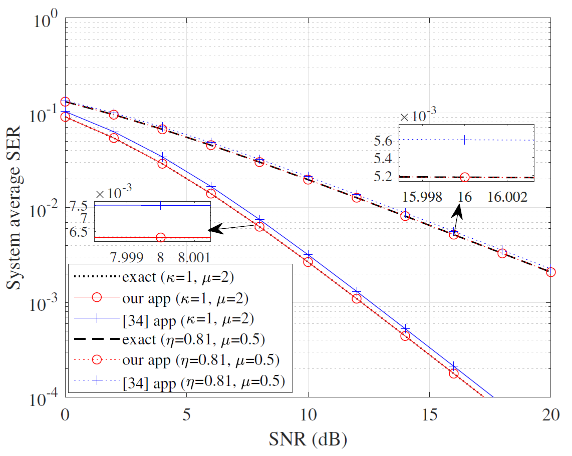
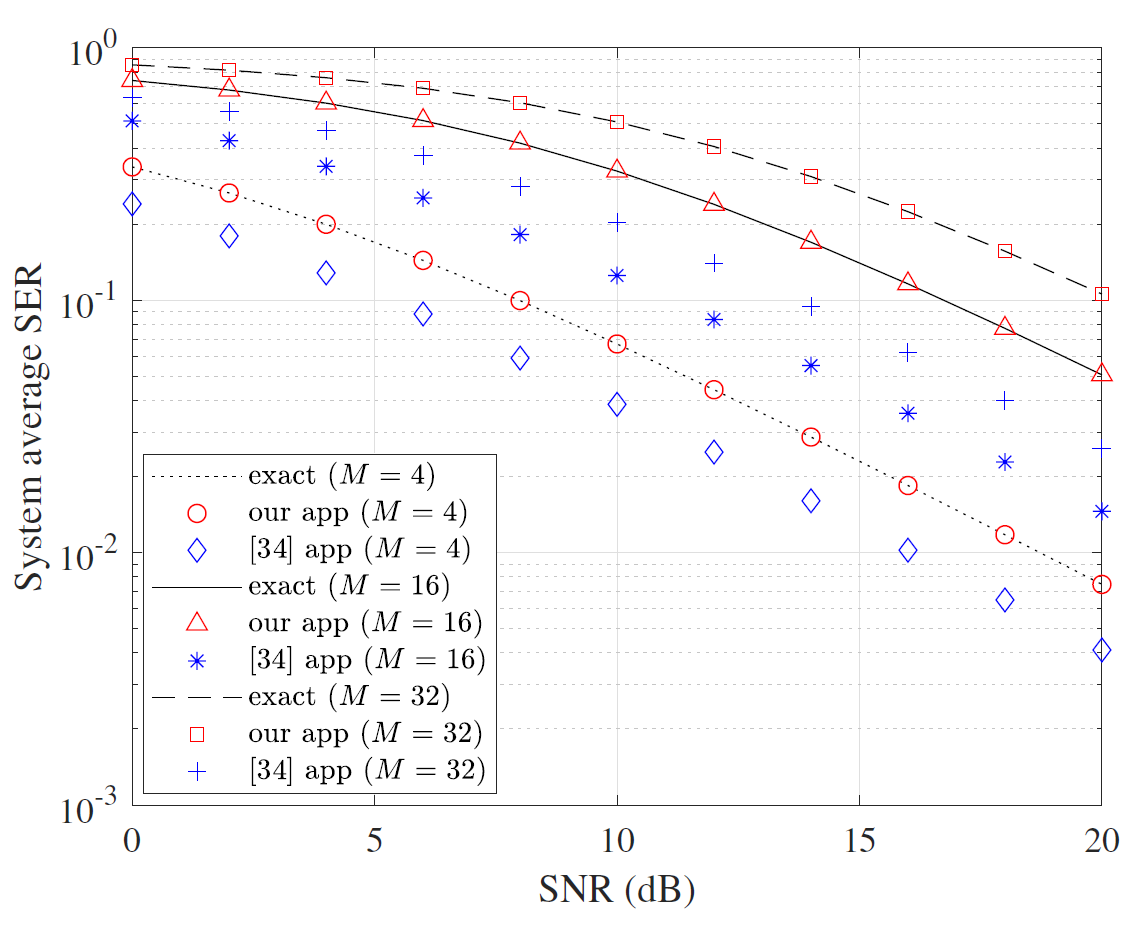
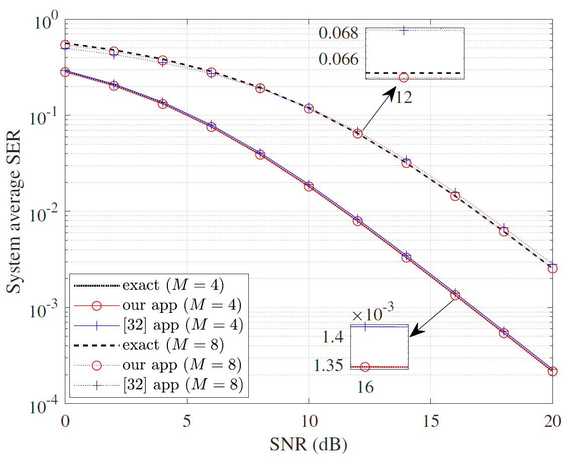
The SER expressions are expressed by [TeX:] $$M G F(\cdot)$$ functions in (38)-(40), in which (39) is given at the bottom of page 10, and we represent SER in terms of the integral relationship between the density function and Q-function in this paper. As shown in Figs. 3–5, we compare our theoretical analyzes with those estimated by the previous methods in [34] and [32]. One can see that our derivation has a very close approximation to the exact SER expression. Fig. 3 compares our derivations with those in [34] under BPSK modulation, showing that both estimates closely align with the exact values. Fig. 4 shows the comparison under M-QAM modulation, and it can be seen that the approximate error in [34] increases with higher-order QAM modulation, while our approximate theoretical values still maintain good consistency with the exact value, which verifies the effectiveness of our derivations. Fig. 5 presents the comparison between our expressions and the expressions derived in [32] underM-PSK modulation, demonstrating close estimations and further validating the accuracy and higher precision of our derivations.

IV. NUMERICAL RESULTS AND DISCUSSIONS

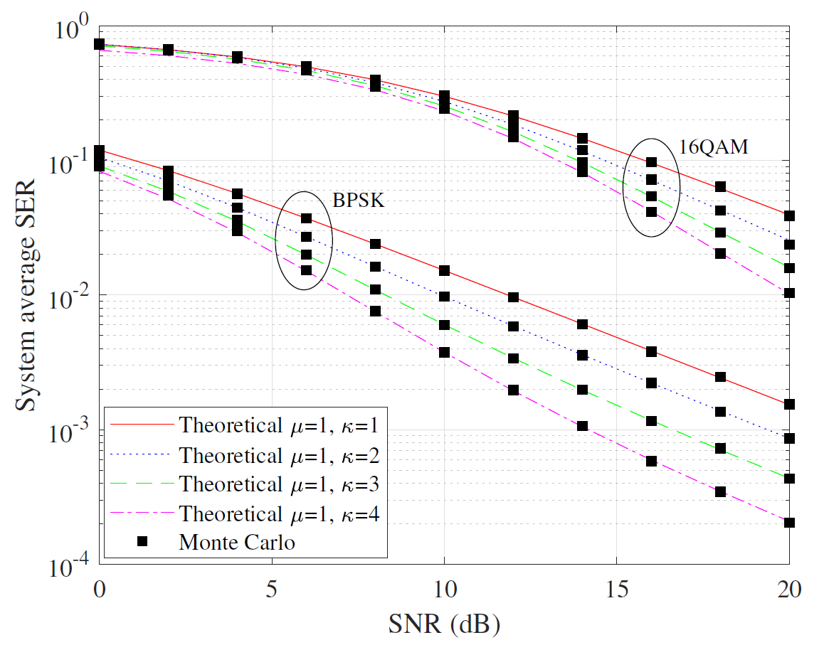
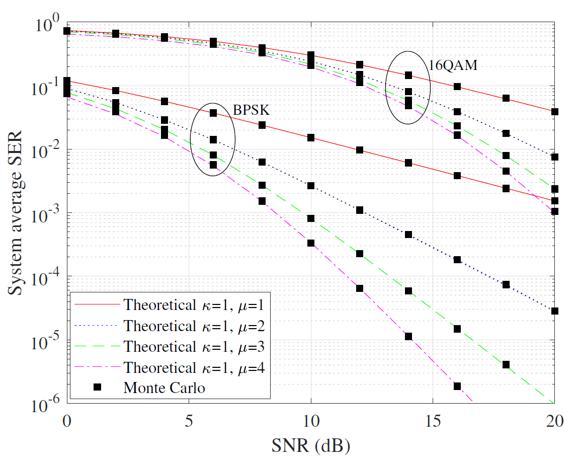
Simulations are conducted to validate the analytical derivations presented in this section. Our analysis of SER performance primarily focuses on two modulation schemes, namely BPSK and 16-QAM. This is because BPSK is one of the most common low-order modulation techniques, whereas 16- QAM is a high-speed digital modulation technique often used in modern communication systems. Furthermore, in MC simulations, [TeX:] $$10^6$$ random samples are generated from the [TeX:] $$\kappa - \mu$$ or [TeX:] $$\eta-\mu$$ distributions by adopting the method described in [34], and the relevant channel coefficients are simulated according to their physical models represented in [50].

To verify the accuracy of our derivation, the theoretical approximations (App) are compared with MC simulations. The MC results are plotted as black square markers in Figs. 6- 10. Overall, our estimated values show good agreement with the MC simulations. Although some values are not perfectly consistent in the low SNR region, the difference is negligible, and this difference can be reduced by increasing the value of the truncation point T. In the high SNR region, the two curves are more closely, thus corroborating the precision of our derivation.

Fig. 6 shows the SER performance with a varying parameter κ in (10). As we observe, the SER performance improves with increasing κ for both modulation schemes. This improvement is due to higher κ values accompanied by a stronger LOS component and less severe fading. Fig. 7 shows the SER versus SNR plot over the [TeX:] $$\kappa - \mu$$ fading channel with the varying number of clusters μ in (11). We observe that as μ increases, the SER decreases. Especially, as depicted in Figs. 6 and 7, when SNR is low, the corresponding SER values for different μ values are quite similar. In high SNR regime, the SER differences for different values of μ are obvious. Moreover, we also see that the App and MC curves keep consistency even if κ and μ change. With identical parameter settings, the SER performance of BPSK modulation consistently outperforms that of higher-order QAM modulation like 16-QAM, expectedly considering the effect of the modulation order on the SER performance.

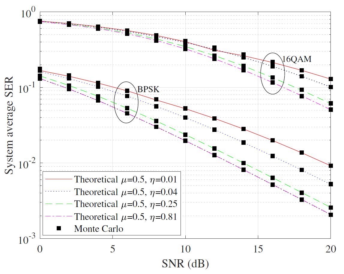
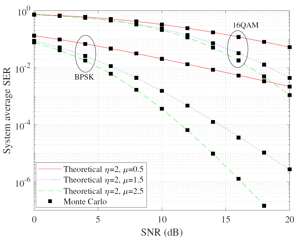
Figs. 8 and 9 are the SER performance results in (20) and (21) for different parameters η and μ, over [TeX:] $$\eta - \mu$$ fading channels. As shown here, when η and μ increase, SER continuously decreases, and the difference between the curves for different parameter values becomes wider with the increase of SNR. In addition, through the above four simulation figures, we can also see that the parameter μ exerts a pronounced influence on the SER metric, underscoring the considerable impact of the multipath factor in the fading channel. Furthermore, we can also observe the influence of fading parameters on the SER accuracy in the low SNR region. The SER corresponding to larger fading parameters is not perfectly aligned with the MC results, which is due to the fading parameters affecting the choice of the optimal truncation parameter T. When the SNR is low, larger fading parameters typically require a larger truncation parameter T to ensure a more accurate SER.

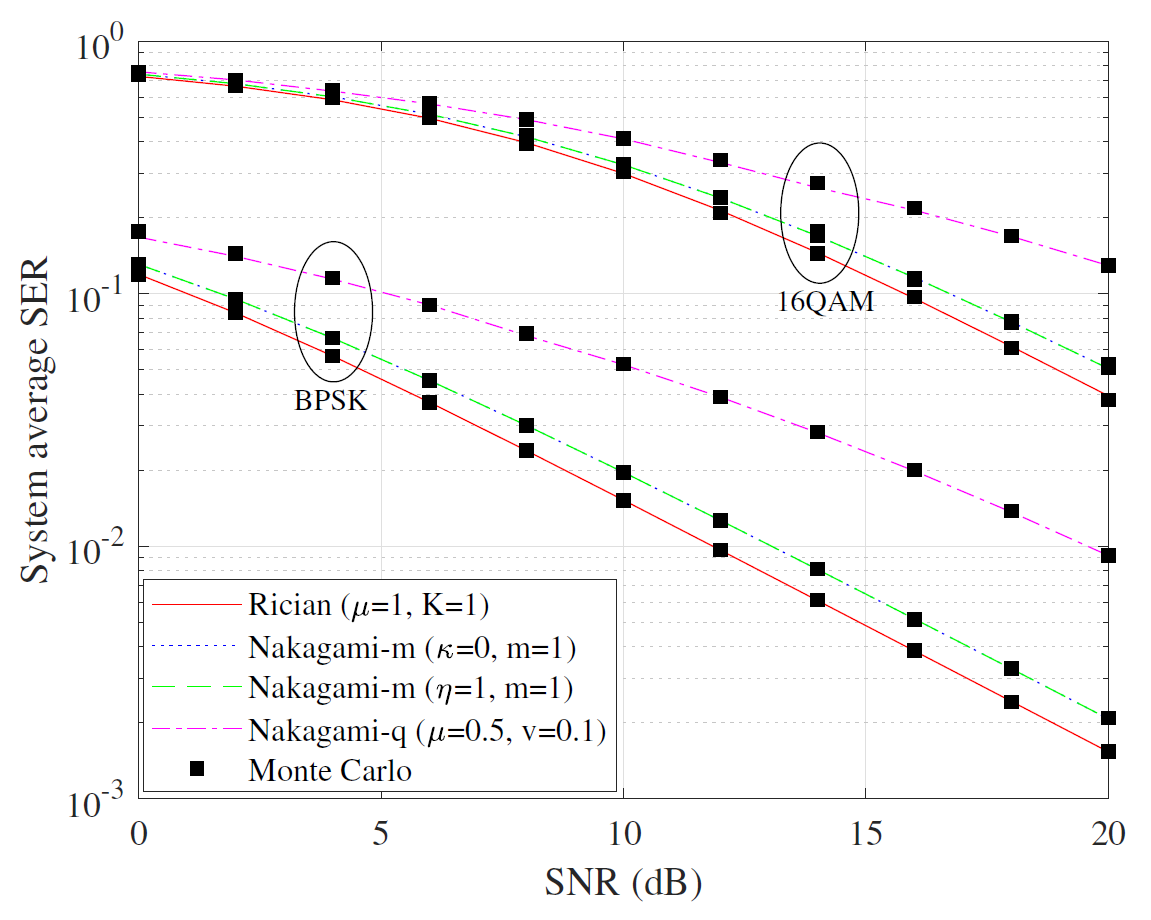
With the generalized expressions we derived, it is easy to obtain the simulation results for SER in several common channels, such as Rician, Nakagami-m and Hoyt, as shown in Fig. 10. One can observe that the blue line and the green line coincide because they correspond to the same Rayleigh channel. It is also worth discovering that the theoretical SER curves and the ones obtained by MC simulation are closely matched, which demonstrates the validity of our analysis.

V. CONCLUSION

In this article, we have derived the simplified closed-form expressions for SER with arbitrary small errors over the generalized [TeX:] $$\kappa - \mu$$ and [TeX:] $$\eta - \mu$$ fading channels. From our analysis, we obtain a conclusion that the dependent truncation parameter T is influenced by the fading channel parameters. In the low SNR region, larger fading parameters require a larger T; conversely, a smaller T is sufficient to deal with smaller channel parameters. Besides, we have demonstrated that the obtained SER expressions are versatile and can characterize SER expressions under different wireless environments. Our analysis was validated by numerical simulations, revealing the accuracy and validity of our derivations. In particular, our derived expressions exhibit higher accuracy compared to the previous methods. Simulation results also demonstrated that the SER performance over [TeX:] $$\kappa - \mu$$ and [TeX:] $$\eta - \mu$$ fading channels can be enhanced by increasing values of parameters [TeX:] $$\kappa, \eta \text{ and } \mu$$ with μ having a more pronounced effect than κ and η.

APPENDIX A

PROOF OF LEMMA 1

According to the original interpretation of SER that appeared in the literature [6], the SER expression under PSK modulation is analyzed as follows,

Since the part involving t is separate from the integral regarding γ, we will simplify the integral regarding γ first. Extract the integral involving γ as [TeX:] $$Z_p=\int_0^{\infty} \gamma^{\mu-1+t} e^{-\left(\frac{\mu(1+\kappa)}{\bar{\gamma}}+\frac{g_p}{\sin ^2 \theta}\right) \gamma} d \gamma,$$ and let [TeX:] $$a=\mu-1+t \text {, }$$ [TeX:] $$b=\frac{\mu(1+\kappa)}{\bar{\gamma}}+\frac{g_p}{\sin ^2 \theta},$$ we further simplify [TeX:] $$Z_p=\int_0^{\infty} \gamma^a e^{-b \gamma} d \gamma$$ as

By plugging [TeX:] $$Z_p$$ into (42), we obtain the new expression as

With an analysis similar to the above, the SER expression under QAM modulation is given as

where [TeX:] $$Z_q=\frac{(\mu+t-1) !}{\left(\frac{\mu(1+\kappa)}{\bar{\gamma}}+\frac{g_q}{\sin ^2 \theta}\right)^{\mu+t}}.$$

APPENDIX B

PROOF OF LEMMA 2

Proof : The remainder after truncating the first T elements of the sum in (5) is expressed as

Obviously, the main cause of the approximation error is the infinite series expression involving t. In this case, by putting the integral and the coefficient part aside, we just focus on the following expression

Since μ, κ and s are constants, [TeX:] $$\frac{1}{\left(\frac{\mu(1+\kappa)}{\bar{\gamma}}+\frac{g_p}{\sin ^2 \theta}\right)^\mu}$$ is also a constant. Let [TeX:] $$V=\frac{\left(\mu^2 \frac{\kappa(1+\kappa)}{\bar{\gamma}}\right)}{\left(\frac{\mu(1+\kappa)}{\bar{\gamma}}+\frac{g_p}{\sin ^2 \theta}\right)},$$ we obtain a new function [TeX:] $$f(t)$$ as

There exists [TeX:] $$t^{\prime}$$ such that the above function [TeX:] $$f(t^{\prime})$$ converges to [TeX:] $$0 \text{ after } t^{\prime}.$$ Moreover, it is observed that [TeX:] $$f(t)$$ can rapidly converge to 0 after [TeX:] $$x^{\prime}$$ by an example of [TeX:] $$f(100)=1.358 \times 10^{-172}.$$

Moreover, assuming that at t = T where [TeX:] $$f(t)$$ nears zero, T denotes the optimal value that satisfies the condition in (8). An threshold, for example, [TeX:] $$\epsilon=10^{-4},$$ can be set to assert that [TeX:] $$f(t)\lt \epsilon \text { for } t \geq T,$$ thereby enabling the precise determination of the optimal T in relation to channel fading parameters. Given that V depends on κ and μ, changes in these parameters correspondingly influence V . A substantial value of V implies that [TeX:] $$V^{t},$$ predominates in [TeX:] $$f(t)$$ until t increases to a point where t! becomes significant. Conversely, a smaller V results in a slower ascent of [TeX:] $$V^{t},$$ with t! rapidly becoming the dominant factor in the reduction of [TeX:] $$f(t).$$ Therefore, larger values of κ and μ, which lead to an increase in V , may necessitate a higher T to ensure [TeX:] $$f(t=T).$$ is sufficiently minimal. In contrast, reduced κ and μ values, leading to a decreased V , allow for a lower T, thereby expediting the reduction of [TeX:] $$f(t).$$

Therefore, the approximate SER expressions for M-PSK and M-QAM modulations over [TeX:] $$\kappa - \mu$$ channel are obtained as

APPENDIX C

PROOF OF LEMMA 3

Proof : Let [TeX:] $$A_0=\frac{\mu^\mu(1+\kappa)^\mu}{\pi e^{\mu \kappa} \bar{\gamma}^\mu}, a=\frac{\mu^2 \kappa(1+\kappa)}{\bar{\gamma}}$$ and [TeX:] $$b=\frac{\mu(1+\kappa)}{\bar{\gamma}},$$ we can rewrite (8) as

Assuming [TeX:] $$f(\theta)=\sum_{t=0}^T \frac{a^t}{t !\left(b+\frac{g_p}{\sin ^2 \theta}\right)^{\mu+t}},$$ we find that [TeX:] $$f(\theta)$$ is bounded on the interval [TeX:] $$\left[0, \frac{M-1}{M} \pi\right] .$$ To achieve the closedform SER expression, numerical integration methods can be adopted. However, we find that under M-QAM modulation, the SER results estimated by methods such as numerical integration using rectangular, trapezoidal, and composite trapezoidal approaches have poor accuracy at low SNR. The exception to this is the interpolation numerical integration method. This disparity can be attributed to the SER expression under M-QAM modulation involving two integral operations, leading to error amplification. Therefore, we adopt Lagrangian interpolation-type numerical integration to obtain the closed form of (8) and (9) here [43]. In the interval [TeX:] $$\left[0, \frac{M-1}{M} \pi\right],$$ insert arbitrarily a number of points [TeX:] $$0=\theta_0\lt\theta_1\lt\theta_2\lt\cdots\lt\theta_i\lt\cdots\lt\theta_{N-1}\lt\theta_N=\frac{M-1}{M}\pi$$ and divide the interval [TeX:] $$\left[0, \frac{M-1}{M} \pi\right],$$ into N small intervals [TeX:] $$\left[\theta_0, \theta_1\right],\left[\theta_1, \theta_2\right], \cdots,\left[\theta_{N-1}, \theta_N\right],$$ the length of each interval is [TeX:] $$\Delta \theta=\frac{M-1}{M N} \pi, \quad \theta_i=i \frac{M-1}{M N} \pi .$$ According to the principle of Lagrangian interpolation-type numerical integration [43], when N is large enough, [TeX:] $$\mathcal{P}_{p s k}^{\kappa-\mu}$$ satisfies

Following the same principle, the SER expressions [TeX:] $$\mathcal{P}_{Q A M}^{\kappa-\mu}$$ for the QAM modulation in this case can also be obtained as

in which [TeX:] $$\theta_q=q \frac{2 \pi}{N}, \theta_{q^{\prime}}=q^{\prime} \frac{4 \pi}{N}, q \in[1, N] \text { and } q^{\prime} \in[1, N].$$

APPENDIX D

PROOF OF LEMMA 4

Proof : Based on the same analysis as in Appendix A, in [TeX:] $$\eta-\mu$$ channel, the SER expression is computed as

After substituting [TeX:] $$Z=\int_0^{\infty} \gamma^{2 \mu+2 t-1} e^{-\left(\frac{2 \mu h^{\prime}}{\bar{\gamma}}+\frac{g_p}{\sin ^2 \theta}\right)} d \gamma=\frac{(2 \mu-1+2 t) !}{\left(\frac{2 \mu h^{\prime}}{\bar{\gamma}}+\frac{g_p}{\sin ^2 \theta}\right)^{2 \mu+2 t}}$$ into the above expression, we further get

By the truncating operator, we further obtain the approximate expression

where [TeX:] $$A_0=\frac{2 \sqrt{\pi} \mu^{2 \mu}\left(2+\eta^{-1}+\eta\right)^\mu}{\pi \bar{\gamma}^{2 \mu}(\mu-1) ! 4^\mu}, a=\frac{\mu\left(\eta^{-1}-\eta\right)}{4 \bar{\gamma}}$$ and [TeX:] $$b=\frac{2 \mu\left(2+\eta^{-1}+\eta\right)}{4 \bar{\gamma}} .$$ Especially, the analysis similar to that in Appendix B finds that fading channels with larger values of η and μ demand a greater T to satisfy higher accuracy requirements for SER. Similar to Appendix C, the closed-form expression in this case is obtained by the numerical integration as

where [TeX:] $$\theta_i=i \frac{M-1}{M N} \pi(i \in[1, N])$$ is represented by [TeX:] $$0\lt\theta_1\lt\theta_2\cdots\lt\theta_N=\frac{M-1}{M}\pi.$$

By the same principle, we can obtain the closed-form SER expression [TeX:] $$\mathcal{P}_{Q A M}^{\eta-\mu}$$ under QAM modulation over the [TeX:] $$\eta - \mu$$ channel, and see the text for the specific formula.

References

- 1 Y . Sun, J. Chen, Z. Wang, M. Peng, and S. Mao, "Enabling mobile virtual reality with open 5G, fog computing and reinforcement learning," IEEE Network, vol. 36, no. 6, pp. 142-149, Dec. 2022.doi:[[[10.1109/MNET.010.2100481]]]
- 2 M. Almekhlafi, M. A. Arfaoui, C. Assi, and A. Ghrayeb, "Superpositionbased URLLC traffic scheduling in 5G and beyond wireless networks," IEEE Trans. Commun., vol. 70, no. 9, pp. 6295-6309, Jul. 2022.doi:[[[10.1109/TCOMM.2022.3194018]]]
- 3 D. Zhang, J. J. P. C. Rodrigues, Y . Zhai, and T. Sato, "Design and implementation of 5G e-health systems: Technologies, use cases, and future challenges," IEEE Commun. Mag., vol. 59, no. 9, pp. 80-85, Oct. 2021.doi:[[[10.1109/MCOM.001.2100035]]]
- 4 J. Yang, A. Aubry, A. De Maio, X. Yu, and G. Cui, "Multi-spectrally constrained transceiver design against signal-dependent interference," IEEE Trans. Sign. Proces., vol. 70, pp. 1320-1332, Jan. 2022.doi:[[[10.1109/TSP.2022.3144953]]]
- 5 Y . M. Eldokmak, M. H. Ismail, and M. S. Hassan, "Secrecy analysis over correlated generalized gamma fading channels," in Proc. IEEE ICCSPA, Cairo, Egypt, Dec. 2022, pp. 1-6.doi:[[[10.1109/ICCSPA55860.2022.10019241]]]
- 6 M. K. Simon and M. S. Alouini, Digital Communication Over Fading Channels. Hoboken, NJ, USA: Wiley-IEEE Press., 2005.custom:[[[-]]]
- 7 K. Jadhav and A. Vidyarthi, "NOMA-spatial modulation: Solving power allocation issue via improved black widow optimization," Advances in Engineering Software, vol. 175, p. 103342, Jan. 2023.doi:[[[10.1016/j.advengsoft.2022.103342]]]
- 8 O. S. Badarneh and M. S. Aloqlah, "Performance analysis of digital communication systems over α − η − µ fading channels," IEEE Trans. Veh. Technol., vol. 65, no. 10, pp. 7972-7981, Oct. 2016.doi:[[[10.1109/TVT.2015.2504381]]]
- 9 J. C. Lin and H. V . Poor, "Optimum combiner for spatially correlated Nakagami-m fading channels," IEEE Trans. Wireless Commun., vol. 20, no. 2, pp. 771-784, Feb. 2021.doi:[[[10.1109/TWC.2020.3028284]]]
- 10 A. Alqahtani, E. Alsusa, A. Al-Dweik, and M. Al-Jarrah, "Performance analysis for downlink NOMA over α -µ generalized fading channels," IEEE Trans. Veh. Technol., vol. 70, no. 7, pp. 6814-6825, Jul. 2021.doi:[[[10.1109/TVT.2021.3082917]]]
- 11 M. D. Yacoub, "Theκ − µ distribution and theη − µ distribution," IEEE Antennas Propag. Mag., vol. 49, no. 1, pp. 68-81, Feb. 2007.doi:[[[10.1109/MAP.2007.370983]]]
- 12 A. Pandey, P. Tiwary, S. Kumar, and S. K. Das, "Fadeloc: Smart device localization for generalizedκ − µ faded IoT environment," IEEE Trans. Sign. Proces., vol. 70, pp. 3206-3220, Jun. 2022.doi:[[[10.1109/TSP.2022.3183527]]]
- 13 M. Hasna and M. S. Alouini, "End-to-end performance of transmission systems with relays over Rayleigh-fading channels," IEEE Trans. Wireless Commun., vol. 2, no. 6, pp. 1126-1131, Nov. 2003.doi:[[[10.1109/TWC.2003.819030]]]
- 14 S. Stein, "Fading channel issues in system engineering," IEEE J. Sel. Areas Commun., vol. 5, no. 2, pp. 68-89, Feb. 1987.doi:[[[10.1109/JSAC.1987.1146536]]]
- 15 W. Xu, J. Zhang, Y . Liu, and P. Zhang, "Performance analysis of semiblind amplify-and-forward relay system in mixed Nakagami-m and Rician fading channels," IEICE Trans. Commun., vol. E93.B, no. 11, pp. 3137-3140, Nov. 2010.doi:[[[10.1587/transcom.E93.B.3137]]]
- 16 K. P. Peppas, G. C. Alexandropoulos, and P. T. Mathiopoulos, "Performance analysis of dual-hop AF relaying systems over mixed η − µ and κ − µ fading channels," IEEE Trans. Veh. Technol., vol. 62, no. 7, pp. 3149-3163, Mar. 2013.doi:[[[10.1109/TVT.2013.2251026]]]
- 17 P. Sharma, A. Kumar, and M. Bansal, "Performance analysis of downlink NOMA over η − µ and κ − µ fading channels," IET Commun., vol. 14, no. 3, pp. 522-531, Feb. 2020.doi:[[[10.1049/iet-com.2019.0413]]]
- 18 Y . Hua, "Generalized channel probing and generalized pre-processing for secret key generation (early access)," IEEE Trans. Sign. Proces., pp. 1-16, Mar. 2023.doi:[[[10.1109/tsp.2023.3259142]]]
- 19 J. Lin et al., "Transmissive metasurfaces assisted wireless communications on railways: Channel strength evaluation and performance analysis," IEEE Trans. Commun., vol. 71, no. 3, pp. 1827-1841, Jan. 2023.doi:[[[10.1109/TCOMM.2023.3239932]]]
- 20 D. Krstic, S. Suljovic, N. Petrovic, S. Minic, and Z. Popovic, "Determining the ABEP under the influence of κ − µ fading and CCI with sc combining at L-branch receiver using moment generating function," in Proc. IEEE SoftCOM, Split, Croatia, Oct. 2022, pp. 1-5.doi:[[[10.23919/SoftCOM55329.2022.9911453]]]
- 21 V . K. Dwivedi and G. Singh, "Moment generating function based performance analysis of maximal-ratio combining diversity receivers in the generalized-K fading channels," Wireless Pers. Commun., vol. 77, no. 3, pp. 1959-1975, Aug. 2014.doi:[[[10.1007/s11277-014-1618-1]]]
- 22 G. Xu et al., "Outage probability and average BER of UAV-assisted dual-hop FSO communication with amplify-and-forward relaying," IEEE Trans. Veh. Technol., vol. 72, no. 7, pp. 8287-8302, Jul. 2023.doi:[[[10.1109/TVT.2023.3252822]]]
- 23 G. Xu and Z. Song, "Performance analysis for mixed κ − µ fading and M-distribution dual-hop radio frequency/free space optical communication systems," IEEE Trans. Wireless Commun., vol. 20, no. 3, pp. 1517-1528, Mar. 2021.doi:[[[10.1109/TWC.2020.3034104]]]
- 24 S. P. Herath, N. Rajatheva, and C. Tellambura, "Unified approach for energy detection of unknown deterministic signal in cognitive radio over fading channels," in Proc. IEEE ICC Wkshps, Jun. 2009, pp. 1-6.doi:[[[10.1109/ICCW.2009.5208031]]]
- 25 A. M. Magableh and M. M. Matalgah, "Moment generating function of the generalized α − µ distribution with applications," IEEE Commun. Lett., vol. 13, no. 6, pp. 411-413, Jun. 2009.doi:[[[10.1109/LCOMM.2009.090339]]]
- 26 A. S. Gvozdarev, "The generalized MGF approach to closed-form average symbol error rate calculation," IEEE Commun. Lett., vol. 25, no. 4, pp. 1124-1128, Apr. 2021.doi:[[[10.1109/LCOMM.2020.3044157]]]
- 27 M. A. Ahmed, A. Baz, and C. C. Tsimenidis, "Performance analysis of NOMA systems over rayleigh fading channels with successiveinterference cancellation," IET Commun., vol. 14, no. 6, pp. 1065-1072, Apr. 2020.doi:[[[10.1049/iet-com.2019.0504]]]
- 28 F. Kara and H. Kaya, "BER performances of downlink and uplink NOMA in the presence of SIC errors over fading channels," IET Commun., vol. 12, no. 15, pp. 1834-1844, Aug. 2018.doi:[[[10.1049/iet-com.2018.5278]]]
- 29 X. Zhang, L. Yang, Z. Ding, J. Song, Y . Zhai, and D. Zhang, "Sparse vector coding-based multi-carrier NOMA for in-home health networks," IEEE J. Sel. Areas Commun., vol. 39, no. 2, pp. 325-337, Feb. 2021.doi:[[[10.1109/JSAC.2020.3020679]]]
- 30 Y . Zhang, K. Xiong, P. Fan, H. Yang, and X. Zhou, "Space-time network coding with multiple AF relays over Nakagami-m fading channels," IEEE Trans. Veh. Technol., vol. 66, no. 7, pp. 6026-6036, Jul. 2017.doi:[[[10.1109/TVT.2016.2627338]]]
- 31 S. Dutta and A. Chandra, "Accurate SER expressions for M-ary dual ring star QAM in fading channels," in Proc. IEEE CODIS, Kolkata, India, Dec. 2012, pp. 1-4.doi:[[[10.1109/CODIS.2012.6422121]]]
- 32 Z. Zhao, G. Xu, N. Zhang, and Q. Zhang, "Performance analysis of the hybrid satellite-terrestrial relay network with opportunistic scheduling over generalized fading channels," IEEE Trans. Veh. Technol., vol. 71, no. 3, pp. 2914-2924, Jan. 2022.doi:[[[10.1109/TVT.2021.3139885]]]
- 33 O. S. Badarneh and R. Mesleh, "Spatial modulation performance analysis over generalized η − µ fading channels," in Proc. IEEE PIMRC, Sep. 2013, pp. 886-890.doi:[[[10.1109/PIMRC.2013.6666262]]]
- 34 B. Kumbhani and R. S. Kshetrimayum, "MGF based approximate SER calculation of SM MIMO systems over generalized η − µ and κ − µ fading channels," Wireless Pers. Commun., vol. 83, no. 3, pp. 19031913, Aug. 2015.doi:[[[10.1007/s11277-015-2493-0]]]
- 35 C. Stefanovic and A. G. Armada, "Performance analysis of doublescattered double-shadowed channel model for UAV-to-ground systems," inProc.IEEEGLOBECOM, Rio de Janeiro, Brazil, pp. 4479-4484, Dec. 2022.doi:[[[10.1109/GLOBECOM48099.2022.10001591]]]
- 36 V . K. Chapala and S. M. Zafaruddin, "Reconfigurable intelligent surface empowered multi-hop transmission over generalized fading," in Proc. IEEE VTC, Helsinki, Finland, Jun. 2022, pp. 1-5.doi:[[[10.1109/VTC2022-Spring54318.2022.9860783]]]
- 37 Z. Zhao, G. Xu, N. Zhang, and Q. Zhang, "Performance analysis of the hybrid satellite-terrestrial relay network with opportunistic scheduling over generalized fading channels," IEEE Trans. Veh. Technol., vol. 71, no. 3, pp. 2914-2924, Jan. 2022.doi:[[[10.1109/TVT.2021.3139885]]]
- 38 N. Bhargav, S. L. Cotton, and D. E. Simmons, "Secrecy capacity analysis over κ − µ fading channels: theory and applications," IEEE Trans. Commun., vol. 64, no. 7, pp. 3011-3024, Jul. 2016.doi:[[[10.48550/arXiv.1506.08606]]]
- 39 M.-T. ElAstal, A. M. Abu-Hudrouss, A. Alhabbash, and G. Kaddoum, "Performance analysis of signed quadrature spatial modulation system over Nakagami-m fading channels with spatial correlation," Physical Commun., vol. 57, p. 101972, Apr. 2023.doi:[[[10.1016/j.phycom.2022.101972]]]
- 40 M. Srinivasan and S. Kalyani, "Secrecy capacity of κ − µ shadowed fading channels," IEEE Commun. Lett., vol. 22, no. 8, pp. 1728-1731, Aug. 2018.doi:[[[10.1109/LCOMM.2018.2837859]]]
- 41 D. Zhang, Y . Liu, L. Dai, A. K. Bashir, A. Nallanathan, and B. Shim, "Performance analysis of FD-NOMA-based decentralized V2X systems," IEEE Trans. Commun., vol. 67, no. 7, pp. 5024-5036, Jul. 2019.doi:[[[10.1109/TCOMM.2019.2904499]]]
- 42 M. Di Renzo, F. Graziosi, and F. Santucci, "Channel capacity over generalized fading channels: A novel MGF-based approach for performance analysis and design of wireless communication systems," IEEE Trans. Veh. Technol., vol. 59, no. 1, pp. 127-149, Jan. 2010.doi:[[[10.1109/TVT.2009.2030894]]]
- 43 D. Kermanschah, "Numerical integration of loop integrals through local cancellation of threshold singularities," J. High Energ. Phys., vol. 2022, no. 151, pp. 1-54, Jan. 2022.doi:[[[10.48550/arXiv.2110.06869]]]
- 44 Z. Wang and G. Giannakis, "A simple and general parameterization quantifying performance in fading channels," IEEE Trans. Commun., vol. 51, no. 8, pp. 1389-1398, Aug. 2003.doi:[[[10.1109/TCOMM.2003.815053]]]
- 45 N. Y . Ermolova and O. Tirkkonen, "The η − µ fading distribution with integer values ofµ ," IEEE Trans. Wireless Commun., vol. 10, no. 6, pp. 1976-1982, Jun. 2011.doi:[[[10.1109/TWC.2011.032411.100638]]]
- 46 S. K. Yoo, S. L. Cotton, P. C. Sofotasios, and S. Freear, "Shadowed fading in indoor off-body communication channels: A statistical characterization using the κ - µ /gamma composite fading model," IEEE Trans. Wireless Commun., vol. 15, no. 8, pp. 5231-5244, Apr. 2016.doi:[[[10.1109/TWC.2016.2555795]]]
- 47 M. Abramowitz, Handbook of Mathematical Functions, With Formulas, Graphs, and Mathematical Tables,. USA: Dover Publications, Inc., 1974.custom:[[[-]]]
- 48 N. Y . Ermolova, "Moment generating functions of the generalizedη − µ andκ − µ distributions and their applications to performance evaluations of communication systems," IEEE Commun. Lett., vol. 12, no. 7, pp. 502-504, Jul. 2008.doi:[[[10.1109/LCOMM.2008.080365]]]
- 49 C. Ben Issaid, M.-S. Alouini, and R. Tempone, "On the fast and precise evaluation of the outage probability of diversity receivers over α − µ , κ − µ , and η − µ fading channels," IEEE Trans. Wireless Commun., vol. 17, no. 2, pp. 1255-1268, Dec. 2018.doi:[[[10.1109/TWC.2017.2777465]]]
- 50 B. Kumbhani and R. S. Kshetrimayum, MIMO wireless communications over generalized fading channels. Boca Raton: CRC Press., 2017.custom:[[[-]]]