Sinuk Choi , Hoseung Song , Eunmin Choi , Jeong-Woo Seo and Ji-Woong Choi
In-vehicle Network Latency Analysis for a Lane Keeping Assistance System
Abstract: Due to the rapid advancements in automotive technologies, vehicles now rely on additional high-speed sensors. This development has led to an increase in transmission rates and traffic levels within in-vehicle networks (IVNs), thereby necessitating changes in the electrical/electronic (E/E) architecture and the emergence of next-generation IVNs. This paper explores the adoption of zonal architecture with an Ethernet backbone as the vehicle topology and analyzes the factors influencing end-to-end latency. Furthermore, to evaluate the impact of IVN latency on safety-critical applications, we adopted the lanekeeping assistance system (LKAS) and employed the widely used metric, lateral error distance, to analyze how much the vehicle deviates from its intended position. We determined the feasibility of LKAS support by establishing vehicle-specific lateral distance thresholds, as allowable lateral error distances vary depending on vehicle size and comparing them with the lateral error distance. Since LKAS demands higher resolutions to achieve enhanced accuracy, this study examines the required resolution for vehicles equipped with next-generation architectures. Additionally, the paper proposes guidelines for the compression ratio of camera sensors at various resolutions and determines the maximum lateral vehicle speed achievable.
Keywords: Advanced driver assistance system , automotive Ethernet , data compression , end-to-end latency , in-vehicle networks , lane-keeping assistance system
I. INTRODUCTION
DUE to the growth of automotive technologies ranging from the advanced driver assistance system (ADAS) to autonomous driving, sensors in vehicles now require highspeed, low-latency data transmission [1]. Traffic of in-vehicle networks (IVNs) has also increased rapidly as many features are added to vehicles. In particular, camera sensors require data rates ranging from approximately 1.6 Gbps to 48 Gbps for fully autonomous driving [2], [3]. However, conventional IVNs such as the controller area network (CAN), controller area network flexible data rate (CAN FD), FlexRay, and mediaoriented systems transport (MOST) provide data rates of up to 1 Mbps, 5 Mbps, 10 Mbps, and 150 Mbps, respectively [4]. There is a limit to handling increased sensor traffic levels with conventional IVNs. Therefore, there is considerable latency in IVNs, which has strongly detrimental effects on safety-related ADAS applications.
To solve this problem, automotive Ethernet and automotive SerDes (serializer/deserializer) technologies are predicted as next-generation IVNs to handle increasing transmission rates. In particular, automotive Ethernet is expected to become a major technology constituting the backbone network of a vehicle because it is compatible with the upper layer of the existing commercial Ethernet technology [5]. A backbone network refers to a major network serving to provide interconnections among various networks in vehicles with high bandwidths. The standardization of automotive Ethernet, providing transmission rates up to 10 Gbps, has been established, and the standard for 25/50 Gbps is currently being established [6].
The automotive electrical/electronic (E/E) architecture is also changing as the number of sensors increases. The conventional automotive E/E architecture follows a decentralized design, consisting of numerous electronic control units (ECUs) distributed throughout the vehicle [7]. Each ECU is responsible for processing data from different sensors, and in cases where additional sensors are required, they must be connected to specific ECUs, even if the distance between the sensor and the ECU is considerable. Consequently, the weight and length of the wiring harness increase due to this functional mapping. Considering these problems, a zonal architecture has been proposed as a next-generation type of E/E architecture for vehicles [8]. In the zonal architecture, sensors are connected to a zonal switch which is positioned at the nearest physical location, as opposed to the use of functional mapping. Therefore, the length and weight of the harness can be decreased. Also, the zonal network is a centralized form of E/E architecture that uses the vehicle’s central computer, meaning that it offers scalability and efficient management of ECUs.
A high transmission rate of the IVN is essential for a backbone network in the zonal architecture, and the development of automotive Ethernet made this possible with the zonal architecture. In reality, most OEMs and suppliers, including BMW, Volkswagen, and Bosch, have announced that they will design their vehicles with the zonal architecture when the Ethernet backbone is applied to vehicles in the future [9].
Therefore, in this paper, we configure the topology of the zonal architecture with an Ethernet backbone in a heterogeneous network and analyze the end-to-end latency encompassing the IVN latency. In addition, to analyze the effects of IVN latency on safety-related applications, a control loop of a lane-keeping assistance system (LKAS) is applied to the IVN configuration of the vehicle. LKAS is one of the most important functions in an ADAS, as it prevents the vehicle from crossing into other lanes.
Furthermore, we employed the broadly used LKAS evaluation metric, lateral error distance, to analyze the impact of IVN latency on the primary autonomous driving function, LKAS. Lateral error distance assists in evaluating the extent to which the vehicle deviates from its intended position [10]–[12]. Considering allowable errors vary with vehicle size, we analyze the feasibility of actual LKAS support by taking into account the maximum allowable lateral distance threshold based on vehicle size. As a result, we provide suitable camera resolutions and compression ratios for practical applications in LKAS that meet the lateral distance threshold conditions.
The main contributions of this paper are listed as follows.
· In this paper, we model end-to-end latency and latency factors, taking into account the recently standardized high transmission speed automotive Ethernet and the zonal architecture proposed for the next-generation E/E structure in vehicles, and present simulation results.
· To analyze the impact of high data transmission rates on IVN latency performance, we considered camera sensor data which is widely used on autonomous vehicles. In particular, we analyze end-to-end latency and dominant latency factors influenced by image data resolution and compression.
· We consider the prominent ADAS feature, LKAS, to analyze the impact of IVN latency on the actual autonomous vehicle. As a result, we analyzed the lateral error distance in LKAS caused by IVN latency and investigated the required compression rates for each resolution based on vehicle size.
II. RELATED WORKS
A. LKAS Model and Methodology
Various studies have been conducted to implement the prominent feature of autonomous vehicles, LKAS. Representatively, S. Wei et al. in [13] categorized various aspects of LKAS, presenting existing research studies corresponding to each category. Moreover, they standardized the objective research evaluation procedure for LKAS and engaged in discussions concerning multiple assessment methodologies. In the research conducted in [14], the authors investigated type 2 fuzzy approaches for lane-keeping assistance systems, considering human drivers. They designed a controller to mitigate uncertainty in the presence of vehicle speed errors. The authors in [15] proposed a driver-centric neural adaptive control-based LKAS model to ensure the smoothness of vehicle control actions and reduce parameter estimation errors. To validate the proposed LKAS model, performance analysis, including speed and lateral offset, was conducted using simulated vehicle dynamics and a driving simulator. In [16], a lane detection method was proposed for estimating the three-dimensional position of drivable lanes. In this study, the proposed method detects whether an object is on the road or off-road and optimally selects weights accordingly. H.-J. Cha et al. demonstrate the impact of the trade-off between the control period and end-to-end latency on LKAS control performance. However, they solely consider latency as an input parameter without analyzing the underlying factors contributing to latency [10].
Many previous LKAS-related studies mostly focused on accurately detecting lanes and reducing vehicle location errors. However, in those studies, IVN latency was not specifically considered in the LKAS control loop. In practical autonomous vehicles, IVN latency is an inevitable occurrence in LKAS. As a result, even when lane detection and vehicle control are executed flawlessly during LKAS application, accidents can potentially occur due to latency in detection or control commands reaching the vehicle, attributed to IVN latency. Therefore, it is imperative to consider IVN latency to ensure the real-time performance of LKAS.
B. IVN Latency Analysis
Many researchers have researched IVN latency since it can result in accidents and vehicle malfunctions. In [17], authors measured the end-to-end latency in a cooperative adaptive cruise control system but overlooked the complexities of vehicle topology with zonal architecture, instead considering a simplistic topology that differs from real-world vehicles. For instance, they do not include gateway latency and artificial intelligence (AI) computing latency in the end-to-end latency calculation due to the simplified vehicle topology. It is crucial to consider a more intricate topology that reflects the network topology of real vehicles since IVN latency increases with the growing number of sensors due to network traffic. In the research conducted in [18], an end-to-end latency performance analysis was conducted, considering domain architecture. In this paper, the authors model end-to-end latency and present latency based on frame size and the number of nodes through analysis and simulation. The authors in [19] proposed a gateway to control data traffic passing through the IVN backbone to prevent transmission efficiency degradation of the IVN Ethernet backbone due to excessive vehicle data traffic and analyzed average latency. Z. Zhou et al. analyzed multiple traffic scheduling and shaping mechanisms in automotive Ethernet. In addition, the authors introduced a time-sensitive networking (TSN)-based test model and analyzed the latency performance [20]. A study conducted in [21] provides an overview of the latency characteristics of IVNs and analysis methods. However, since only up to 1 Gbps Ethernet is considered, high-speed data transmission such as high-definition camera sensor data can be difficult.
While numerous studies have investigated end-to-end IVN latency and latency factors, most of these studies have either considered small-scale data or focused on specific latency factors, resulting in limited findings. Additionally, there has been a lack of performance analysis concerning high data rate Ethernet, as well as zonal architectures in next-generation E/E systems. However, considering the recent standard of Ethernet and sensor data with high data rate in zonal architectures, there is a growing need for latency performance analysis to support the advanced autonomous driving function. Therefore, the study on latency performance analysis considering high data rate is meaningful.
Therefore, we analyze the end-to-end latency and latency factors considering the LKAS operation according to the camera resolution and compression within an IVN. Also, we configure an IVN topology that closely resembles a real vehicle with various transmission rate of the Ethernet backbone network. It is crucial for vehicle network designers to determine the appropriate transmission rate of the backbone, considering the trade-off between performance and cost. A higher transmission rate in the network backbone comes with increased expenses, while a lower rate may fail to meet safety requirements. Accordingly, we provide results concerning the end-to-end latency associated with sensor resolution, along with the required compression ratio.
III. THE EFFECT OF END-TO-END IVN LATENCY IN LKAS
An LKAS, a representative function of an ADAS, is a system that prevents the vehicle from deviating from its lane without human control. The LKAS is mainly composed of a camera sensor, a steering direction sensor, a vehicle speed sensor and a motor-driven power steering (MDPS) [10]. The MDPS is an actuator that controls the heading angle in an LKAS. The operational process of an LKAS is divided into perception, decision, and control processes. In the perception process, both lanes are recognized through the camera sensors and the vehicle states are identified with the steering direction and vehicle speed sensor. Then, sensor data is sent to the vehicle computer (VC). During the decision process, the VC calculates the lateral deviation of the vehicle relative to both lanes with the camera data and determines the heading angle considering the present speed and steering direction of the vehicle. Finally, in the control process, control data is sent to the MDPS to actuate the steering wheel so as to ensure that the vehicle does not deviate from its lane.
TABLE I
| Latency factor | Description |
|---|---|
| [TeX:] $$D_{S 2 V}$$ | Latency from sensor to VC |
| [TeX:] $$D_{V 2 M}$$ | Latency from VC to MDPS |
| [TeX:] $$D_{IVN, S2V}$$ | IVN latency in [TeX:] $$D_{S2V}$$ |
| [TeX:] $$D_{Proc, S2V}$$ | Processing latency in [TeX:] $$D_{S2V}$$ |
| [TeX:] $$D_{IVN, V2M}$$ | IVN latency in [TeX:] $$D_{V2M}$$ |
| [TeX:] $$D_{Proc, V2M}$$ | Processing latency in [TeX:] $$D_{V2M}$$ |
| [TeX:] $$D_T$$ | Transmission latency |
| [TeX:] $$D_F$$ | Frame division latency |
| [TeX:] $$D_P$$ | Propagation latency |
| [TeX:] $$D_G$$ | Gateway latency |
| [TeX:] $$D_S$$ | Switch latency |
| [TeX:] $$D_D$$ | Disrupter latency |
| [TeX:] $$D_Q$$ | Queueing latency |
| [TeX:] $$D_L$$ | LKAS processing latency |
| [TeX:] $$D_C$$ | Compression latency |
During the entire process, the end-to-end latency, meaning the time from sensing to actuation, affects the control performance. Table 1 summarizes the latency factors comprising end-to-end latency. Therefore, the end-to-end latency, [TeX:] $$D_{E 2 E},$$ can be determined as follows:
where [TeX:] $$D_{S 2 V}$$ is the latency from the sensor to the VC and [TeX:] $$D_{V 2 M}$$ is the latency from the VC to the MDPS. The VC calculates a suitable heading angle that ensures that the vehicle does not deviate from its lane with the received vehicle state data considering that it is the present vehicle state data. However, the VC makes a control decision with previous sensor data if [TeX:] $$D_{S 2 V}$$ is large. Also, the steering wheel is actuated on a latency if [TeX:] $$D_{V 2 M}$$ is large. Therefore, accurate control is ensured only when [TeX:] $$D_{E 2 E}$$ is short enough [10]. The latencies in (1) are composed of the IVN latency and the processing latency. [TeX:] $$D_{S 2 V}$$ can be determined by
where [TeX:] $$D_{I V N,S 2 V}$$ and [TeX:] $$D_{{Proc }, S 2 V}$$ are correspondingly the IVN latency and the processing latency in [TeX:] $$D_{S 2 V}.$$ [TeX:] $$D_{V 2 M}$$ is determined as
In this equation, [TeX:] $$D_{I V N,V 2 M}$$ and [TeX:] $$D_{{Proc },V 2 M}$$ are respectively the IVN latency and the processing latency in [TeX:] $$D_{V 2 M}.$$
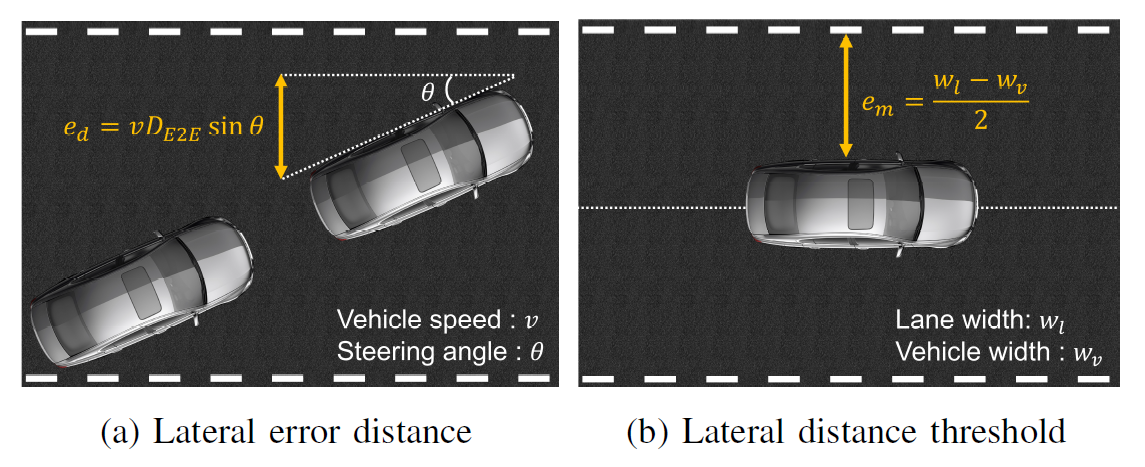
It is possible to calculate how much the vehicle moves in the lateral direction considering [TeX:] $$D_{E 2 E},$$ the heading angle, and the speed of the vehicle (see Fig. 1(a)). The lateral error distance, [TeX:] $$e_d,$$ is computed as
where θ is the heading angle of the vehicle and v is the longitudinal speed of the vehicle. Vehicles supporting LKAS can provide assistance for speeds of up to 200 km/h [22]. There is limited information on LKAS adaptation to other types of transportation. Recently, Honda has been preparing for the development of LKAS for motorcycles [23]. However, the maximum speed for LKAS application on motorcycles has not been specified. Currently, Honda’s LKAS can support speeds of approximately up to 145 km/h [24]. Consequently, when considering LKAS application in vehicles, it must meet more stringent requirements compared to applying it to motorcycles, given the higher LKAS requirements for vehicle use. Therefore, we assumed that v can be supported in the range of 0–200 km/h, and θ is considered to have a range of 0–20 degrees because the ADAS application avoids abrupt directional control of the steering wheel [22].
The maximum allowable error distance of [TeX:] $$e_d$$ is the distance between the lane and the vehicle assuming that the vehicle is at the center of the lane (see Fig. 1(b)). This is determined by considering the width of the vehicle and the lane. Therefore, the lateral distance threshold, [TeX:] $$e_m,$$ is computed as follows:
where [TeX:] $$w_v \text{ and }w_l$$ are the widths of the vehicle and lane, respectively, which can be determined based on Korean road traffic laws, rules for road structure and facilities standards [25]. There are four types of vehicles in Korean law: Passenger vehicles, small vehicles, large vehicles, and semi-trailers. Widths for small and large vehicles are used in this paper (2 m for small vehicles and 2.5 m for large vehicles). Taking an example with a real vehicle model, the width of Hyundai “SANTA FE” is about 1.9 m and Hyundai “Xcient” is 2.5 m [26], [27]. Also, [TeX:] $$w_l$$ is designed considering the vehicle speed, which is assumed to be 3 m, 3.25 m, and 3.5 m for roads with speed limits of 60 km/h, 100 km/h, and more than 100 km/h, respectively. In this case, [TeX:] $$w_l$$ is set to 3.5 m to consider all available vehicle speeds. Therefore, the evaluation criteria for the effects of [TeX:] $$D_{E2E}$$ on the LKAS system can be determined by comparing [TeX:] $$e_d \text{ and }e_m.$$ It is assumed that there is a straight road and the vehicle is always in the middle point of the road. In addition, we assumed that when [TeX:] $$e_d \text{ and }e_m$$ and fails to satisfy the threshold condition, the vehicle would cross into another lane, potentially leading to a collision. In other words, when the lateral distance error exceeds the lateral distance threshold, it indicates that the vehicle is deviating from its current lane center and represents a potential collision risk.
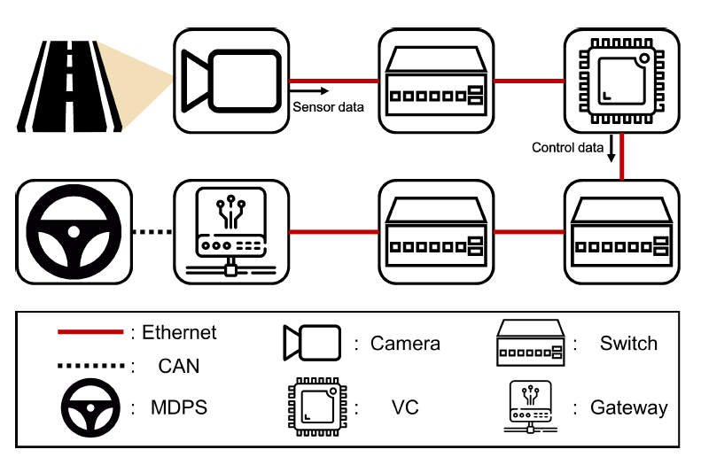
Fig. 2 illustrates an example of the IVN topology considering the LKAS control loop. The camera sensor captures data from the road with lanes and transmits it to the VC connected through automotive Ethernet with a switch. Subsequently, for LKAS, the VC generates control data related to steering angle, speed, and more based on lane and vehicle position and status. The control data is then relayed to the MDPS through a series of switches via the Ethernet-CAN gateway.
A. IVN Latency Factors
First, the factors of [TeX:] $$D_{IVN}$$ of the LKAS control loop are analyzed. [TeX:] $$D_{IVN}$$ contains the transmission latency ([TeX:] $$D_T$$), the frame division latency ([TeX:] $$D_F$$), the propagation latency ([TeX:] $$D_P$$), the gateway latency ([TeX:] $$D_G$$), the switch latency ([TeX:] $$D_S$$), the disrupter latency ([TeX:] $$D_D$$), and the queuing latency ([TeX:] $$D_Q$$). The parameters used to define the latency factors are presented in Table 2.
TABLE II
| Parameters | Description |
|---|---|
| [TeX:] $$e_d$$ | Lateral error distance |
| [TeX:] $$e_m$$ | Lateral distance threshold |
| v | Longitudinal speed of the vehicle (0–2 km/h) |
| θ | Heading angle of the vehicle ([TeX:] $$0-20^{\circ}$$) |
| [TeX:] $$w_v$$ | Width of the vehicle |
| [TeX:] $$w_l$$ | Width of the lane |
| L | The data size of the video sensor |
| R | Data rate of IVN (0–25 Gbps) |
| [TeX:] $$L_f$$ | Length of IVN frame |
| [TeX:] $$L_p$$ | Length of maximum payload |
| [TeX:] $$d_w$$ | Length of the wire (1–1.5 m) |
| s | Propagation speed in wire |
| c | Speed of light ([TeX:] $$3 \cdot 10^8 \mathrm{~m} / \mathrm{s}$$) |
| [TeX:] $$N_D$$ | Number of disrupters in the control loop (0–1) |
| [TeX:] $N_f$$ | Number of arrived frames per second (0–900) |
| [TeX:] $$t_f$$ | Time to extract the lane feature for 1 bit (0.02 ms) |
| [TeX:] $$t_s$$ | Time to calculate the steering angle (7 ms) |
| C | Compression ratio of the data (0–100%) |
| [TeX:] $$t_c$$ | Time to compress/decompress 1 bit (0.029 ns) |
| [TeX:] $$N_{hop}$$ | Hop count in the control loop |
1) Transmission latency : The transmission latency is the length of time required to push all of the packet’s bits into the wire. This latency arises between the Ethernet backbone and the transmitter, which is the camera sensor or VC used when transmitting the data. The transmission latency, [TeX:] $$D_T$$, is determined via
where L is the length of the transmitting data and R is the data rate of the IVN. L is determined according to the pixel size and pixel depth of the camera sensor. This latency significantly differs according to the transmission rate of the Ethernet backbone transmitting the data.
2) Frame division latency : The frame division latency is generated in addition to [TeX:] $$D_T$$ if the data length to be sent exceeds the maximum payload of the IVN frame. For example, considering the Ethernet frame, data exceeding 1500 bytes must be divided into several Ethernet frames and transmitted. Therefore, additional latency is generated by Ethernet frame data apart from the payload data, i.e., overhead of Ethernet frame. An additional 42 bytes overhead except for the payload data will be added per frame. Therefore, frame division latency, [TeX:] $$D_F$$, is computed as
where [TeX:] $$L_f$$ is the length of IVN frame containing overhead and payload, [TeX:] $$L_p$$ is the length of the maximum payload in IVN frame, and [TeX:] $$\lceil\cdot\rceil$$ denotes a ceiling function.
3) Propagation latency : The propagation latency, [TeX:] $$D_P$$, is the length of time taken for a signal to reach its destination through a wire. It is determined via
where [TeX:] $$d_w$$ is the length of the wire and s is the propagation speed in the wire. In copper wire, the speed s is generally 2c/3, where c is the speed of light.
4) Switch latency : The switch latency, [TeX:] $$D_S,$$ is the length of time taken inside the switch, including the routing latency. While it is different for each manufacturer, it generally does not exceed [TeX:] $$10 \mu \mathrm{s}$$ in industrial applications which is very marginal compared to other latencies. There is a variation in this latency, so the mean value of specific switch model is used in this paper for analysis. As an example, [TeX:] $$D_S$$ is set to the mean value of RSG2288, which is [TeX:] $$7 \mu \mathrm{s}$$ [28]. It is also assumed that switches always have the same latency regardless of message types for simple analysis.
5) Gateway latency : The gateway latency, [TeX:] $$D_G,$$ is the length of the time taken inside the gateway. [TeX:] $$D_G$$ includes the routing, buffering, and transforming latency. Similar to [TeX:] $$D_S$$, [TeX:] $$D_G$$ varies among manufacturers and exhibits variations. Taking [29] as an example, [TeX:] $$D_G$$ is set to [TeX:] $$500 \mu \mathrm{s}$$, representing the mean value of gateway latency observed in the implemented Ethernet-CAN gateway discussed in [29]. Gateway latency typically surpasses switch latency as it encompasses both routing and transforming processes. Additionally, it is assumed that gateways consistently exhibit the same latency irrespective of message types.
6) Disrupter latency : The disrupter latency, [TeX:] $$D_D,$$ is the latency that occurs in the switch when two or more sensors with the same priority are contained in the control loop. It is computed as
where [TeX:] $$N_D$$ is the number of disrupters in the control loop. Camera data for the LKAS should be transmitted with the same level of priority for accurate perceptions, and this causes disrupter latency in the switch. If only one camera is in the control loop, [TeX:] $$N_D$$ is zero. However, if two cameras (i.e., stereo) with the same priority are in the control loop, [TeX:] $$N_D$$ becomes one and the time is delayed with [TeX:] $$D_T \text{ and} D_F$$ by the disrupter. In this paper, it is assumed that all cameras have the same payload size as it is a stereo type camera.
7) Queuing latency : The queuing latency, [TeX:] $$D_Q,$$ depends on the number of earlier-arriving packets and the waiting time for transmission on the link [30]. This latency considers the delay caused by the nodes connected to the switch, except the camera nodes. The average queuing latency can be computed as shown below.
Here, [TeX:] $$N_f$$ is the number of frames arriving every second. The queuing latency in the network actually takes from micro-seconds to milliseconds.
B. Processing Latency Factors
In addition to [TeX:] $$D_{IVN},$$ the factors of [TeX:] $$D_{Proc},$$ of the LKAS control loop are analyzed. [TeX:] $$D_{Proc, S2V}$$ consists of the AI processing latency, [TeX:] $$D_L,$$ and the compression latency, [TeX:] $$D_C.$$
1) LKAS processing latency : The LKAS processing latency, [TeX:] $$D_L,$$ is the latency in the VC that arises when calculating a suitable heading angle at which lane crossing does not occur. [TeX:] $$D_L$$ includes the time required to identify the lateral deviation of the vehicle from the center of the lane with feature extraction and to calculate the proper heading angle considering the present vehicle speed and steering direction. The latency of feature extraction with AI is usually proportional to the camera data size [31], [32]. Compared to feature extraction, the latency for calculating the heading angle is not proportional to the input data size because the heading angle is calculated with the lateral distance of the vehicle after receiving all the data. Then, [TeX:] $$D_L$$ is determined as
In this equation, [TeX:] $$t_f$$ is the time required to extract the lane feature for 1 bit, and [TeX:] $$t_s$$ is the time required to calculate the proper heading angle. [TeX:] $$D_L$$ differs according to the feature extraction model and the angle calculating algorithm. In this paper, [TeX:] $$t_f$$ and [TeX:] $$t_s$$ are respectively set to 0.02 ns and 7 ms, which are the mean values for extracting the lane feature and calculating the proper heading angle in [31].
2) Compression latency : Compression latency refers to the duration required to compress or decompress data when necessary, typically due to large data sizes. In this paper, we assume that the time required for decompression is the same as that for compression. When compression is necessary, compression latency occurs in the compression module of the camera sensor for compression and in the video codec (VC) for decompression. Accurately modeling compression latency can be challenging due to various factors such as computing power, group of pictures (GOP) size, compression model, coding mode, and input data [33]. However, it is evident that compression latency increases significantly with larger data sizes. Therefore, in this study, we model the compression latency as linearly increasing with the data size. Specifically, we target the H.264 video compression for modeling compression latency since it is currently one of the most widely used video codecs, particularly in vehicular communications [34]. H.264 employs inter-frame compression, and the compression latency increases as the compression ratio rises according to the GOP size. Considering this linear modeling approach, we compute the compression latency, [TeX:] $$D_C,$$ as
where C is the compression ratio of the data (in percentage) and [TeX:] $$t_c$$ is the time required to compress or decompress 1 bit (in seconds). [TeX:] $$t_c$$ is computed based on level 6.2 of H.264, which is the highest level of advanced video coding (AVC) [35]. Here, a maximum of 2.1 GB can be compressed with a compression ratio of 2% for one second. Considering this, [TeX:] $$t_c$$ can be computed as 0.029 ns. [TeX:] $$D_C$$ may increase to the millisecond range depending on the size of the compressed data. H.264 uses lossy compression and thus data compression should be considered carefully because information losses can occur compared to the raw data, even with the same resolution.
There is also control latency for the operation of a steering wheel in LKAS, but it is not considered because it is significantly shorter than others. Considering all types of IVNs and processing latencies, [TeX:] $$D_{S2V}$$ is computed as
(13)
[TeX:] $$\begin{aligned} D_{S 2 V}= & D_C+D_{T_{e t h}}+D_{F_{e t h}}+D_p+D_{D_{E t h}} \\ & +N_{h o p}\left(D_s+D_p\right)+D_Q . \end{aligned}$$Similarly, [TeX:] $$D_{V2M}$$ is computed as
(14)
[TeX:] $$\begin{aligned} D_{V 2 M}= & D_C+D_L+D_{T_{e t h}}+N_{h o p}\left(D_s+D_p\right) \\ & +D_p+D_G+D_{T_{C A N}}+D_P+D_Q . \end{aligned}$$In this equation, [TeX:] $$N_{hop}$$ denotes the hop count, which refers to the number of network devices through the control loop. Note that [TeX:] $$D_T, D_F, D_D \text {, and } D_C$$ are the latency factors that are greatly affected by the data size of the camera. The other latency types do not change dramatically with the data size. When the data size is small, [TeX:] $$D_L$$ is the most significant latency factor. However, as the data size increases, the IVN latency increases and becomes the major latency source of end-toend latency. Therefore, [TeX:] $$D_T, D_F, D_D, D_C, \text { and } D_L$$ can be regarded as the major factors of end-to-end latency of the LKAS.
IV. PERFORMANCE EVALUATION
Fig. 3 shows the designed IVN configuration for the performance evaluation with a topology employing the zonal architecture equipped with an Ethernet backbone. Given that IVN topologies vary depending on the vehicle model, it is challenging to encompass all possible topologies. Therefore, in this paper, we designed the topology with consideration for the LKAS application which includes camera sensors, a VC, and an MDPS. The number of camera was determined by referencing Tesla’s product models, with Tesla Model 3, Model S, Model X, and Model Y using approximately 8–9 cameras [36]. Furthermore, Tesla Semi and Tesla Cybertruck are considering the use of 10 and at least 8 cameras, respectively [37], [38]. Therefore, we assumed the use of 10 cameras, considering the feasibility of applying zonal architecture in future vehicles, and accordingly, we arranged switches and gateways. Similarly, the number of switches in the IVN’s topology is also variable depending on vehicle design and model. As the number of switches increases, routing becomes more complex, and paths lengthen, yet coping with delays due to bottlenecks becomes easier. Conversely, reducing the number of switches simplifies routing, but in cases of bottleneck-induced latency, coping becomes challenging due to the limited number of switches available. Typically, 6–8 zonal switches are considered in a general zonal architecture [39]. Consequently, we employed six switches in our topology, aligning with Toshiba’s considerations [40]. Through this topology, our analysis provides insights into the impact on ADAS encompassing the latency implications associated with zonal networks. Each switch is connected using a 1 m Ethernet wire capable of link speeds of 5, 10, and 25 Gbps, while all of the CAN and Ethernet nodes are connected via a 1.5 m wire.
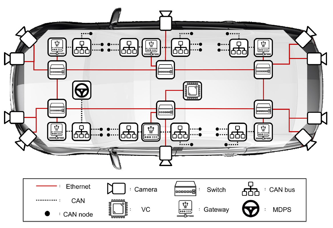
The number of CAN nodes is determined considering ISO11898 [41]. One to two CAN buses are connected to a switch, with each CAN bus containing three to seven CAN nodes. There are 126 CAN messages with different IDs, and the payload of all CAN messages is set to 8 bytes. Regarding the sensor period, the period of the control message to MDPS was set to 10 ms, and sensor messages are equivalently set to 50 ms. For the Ethernet node, two to three Ethernet camera nodes are deployed per switch. The payloads of these camera sensors vary depending on the resolution and are determined as the product of the pixel size and the pixel depth. Here, the pixel size refers to the product of the horizontal and vertical pixels. The pixel depth means the number of colors that one pixel can represent. HD, FHD, QHD, UHD, and 8K are considered for the resolution, and the real color depth of 24 bits is applied for the pixel depth. For the sensor period, the periods of the camera sensors are set to 33.3 ms and 16.7 ms, indicating a 30 fps and 60 fps camera, respectively.
A. The End-to-End IVN Latency with Raw Camera Sensor Data
We analyzed the latency performance based on the sensor resolution of raw camera data and Ethernet backbone transmission rate using the previously defined end-to-end latency and latency factors. When using the raw camera data, [TeX:] $$D_C$$ is omitted. Therefore, if the Ethernet backbone transmission rate is sufficient, it can also provide an advantage in endto- end latency performance. Besides the analysis, computer simulations were also conducted using OMNeT++, a network simulator capable of implementing an IVN in-vehicle network system on a computer. The simulations aimed to validate the analysis results, verify the latency in each sensor data, and design the configuration of the desired IVN topology [42].
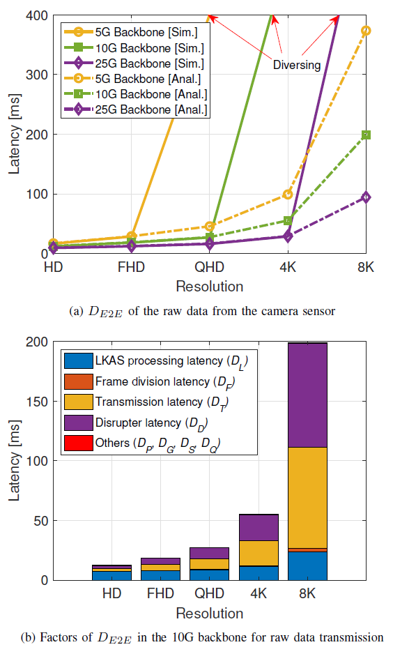
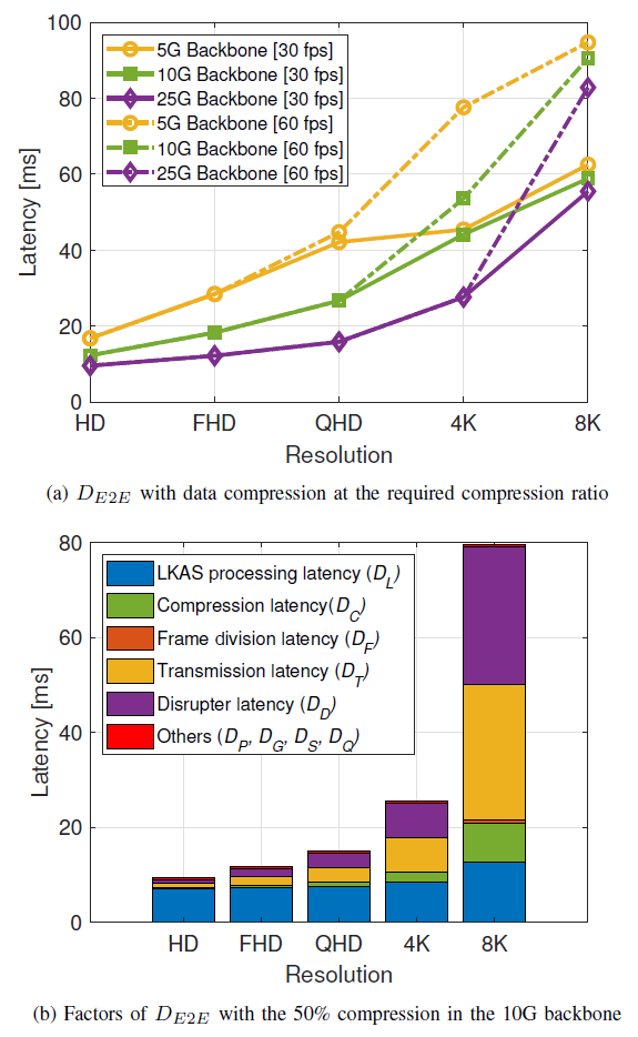
First, [TeX:] $$D_{E2E}$$ of the camera sensors for each resolution without compression was calculated based on (1)–(13) with the different Ethernet backbones of 5G, 10G, and 25G (see Fig. 4(a)). [TeX:] $$D_{E2E}$$ increases when the data size increases with a higher resolution and when an Ethernet backbone with low link rate is used. We find that [TeX:] $$D_{E2E}$$ is significantly affected by the link rate of the Ethernet backbone. For example, [TeX:] $$D_{E2E}$$ with 8K resolution varies from 100 ms for 25G backbone to 370 ms for 5G backbone. Unlike the analysis, which utilized average latency values in queuing, switching, and disruption calculations, the simulation results incorporated the effects of statistical variables. It is important to note that the simulation results exhibit similar performance to the analytical results, with negligible variations from the mean values. This suggests that the random effects on latency are currently marginal in the given scenarios, except for extreme cases where the latency increases without bounds over time (e.g., in scenarios involving QHD for 5G, 4K for 10G, and 8K for 25G backbones). To ensure easier readability and avoid redundancy, simulation results are not presented in the subsequent graphs since they align closely with the analytical findings.
To analyze the effects on each of the latency factors, the proportion of each latency factor in the 10G Ethernet backbone is shown as an example in Fig. 4(b). It is clear that [TeX:] $$D_{E2E}$$ does not change dramatically when the resolution of the camera is low because [TeX:] $$D_{Proc}$$ is the most significant latency factor. However, as the resolution increases, [TeX:] $$D_{E2E}$$ changes remarkably because [TeX:] $$D_{IVN}$$ increases and becomes the major latency source of [TeX:] $$D_{E2E}$$. In particular, [TeX:] $$D_T, D_F, \text { and } D_D$$ are greatly affected by the data size of the camera, having considerable effects on [TeX:] $$D_{E2E}$$.
B. The End-to-End Latency with Compressed Camera Sensor Data
We analyzed the end-to-end latency performance of the compressed camera sensor data similar to raw camera sensor data. Compression reduces data size but introduces necessary compression latency, thus affecting end-to-end latency performance. Firstly, we consider data loss for the camera sensor. If [TeX:] $$D_T$$ of the camera exceeds the sensor period of the camera (i.e., 33.3 or 16.7 ms), data loss occurs because the transmission of the new frame starts before the transmission of the previous frame ends. Therefore, it is necessary to check whether [TeX:] $$D_T$$ is smaller than the sensor period. To prevent this type of data loss, compression of the sensor data should be considered. Table 3 shows the required minimum compression ratio to prevent the loss of data. Fig. 5(a) shows [TeX:] $$D_T$$ after data compression with the required compression ratio. We found that the [TeX:] $$D_T$$ values of the camera sensors are smaller than the sensor period, becoming similar when data is compressed by the required compression ratio for resolutions with the values in Table 3. Here, [TeX:] $$D_C$$ occurs simultaneously and affects [TeX:] $$D_T$$. It also differs according to the compressed data size. The compressed data size becomes larger when the resolution increases or the compression ratio decreases. Fig. 5(b) shows [TeX:] $$D_C$$ with the required compression ratio. We find here that the compression latency, [TeX:] $$D_C,$$ increases when the size of the compressed data is large.
TABLE III
| Camera specification | Required compression ratio [%] | |||
|---|---|---|---|---|
| Sensor period | Resolution | 5G Backbone | 10G Backbone | 25G Backbone |
| 30 fps | HD, FHD | 0 | 0 | 0 |
| QHD | 0 | 0 | 0 | |
| 4K | 23.15 | 0 | 0 | |
| 8K | 80.92 | 61.83 | 4.55 | |
| 60 fps | HD, FHD | 0 | 0 | 0 |
| QHD | 8.38 | 0 | 0 | |
| 4K | 61.58 | 23.15 | 0 | |
| 8K | 90.46 | 80.92 | 52.28 | |
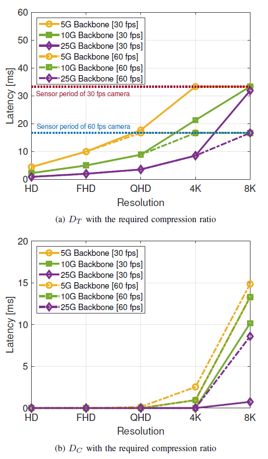
Fig. 6 presents [TeX:] $$D_{E2E}$$ and latency factors after video compression with 50% compression ratio. As shown in Fig. 6(a), [TeX:] $$D_{E2E}$$ of compressed data has lower latency when compared to [TeX:] $$D_{E2E}$$ of raw data. The data size of the camera sensor decreased significantly after compression, resulting in an effective reduction in IVN latency. Consequently, the end-to-end latency decreased compared to the raw camera sensor data for all Ethernet backbone transmission rates. Fig. 6(b) shows latency factors in the 10G backbone. When compared with Fig 4(b), [TeX:] $$D_C$$ for video data compression was added. However, due to the reduced data rate, the latency required in the backbone and the latency related to image processing are reduced, resulting in a reduction in [TeX:] $$D_{E2E}$$. It can be seen that [TeX:] $$D_C$$ is not zero when compression is required for a higher resolution to meet the requirement of the transmission latency being smaller than the sensor period. Also, we find that other latency factors which are proportional to the data size are affected by compression.
C. Latency Effects on LKAS Performance
We considered [TeX:] $$e_d \text{ and } e_m$$ to investigate the feasibility of LKAS support. If [TeX:] $$e_d$$ exceeds [TeX:] $$e_m,$$ it indicates the potential for lane departure beyond the lateral distance threshold, making it challenging to provide LKAS functionality. Fig. 7 shows the maximum [TeX:] $$e_d$$ of the vehicle with the maximum longitudinal speed, i.e., v is 200 km/h and [TeX:] $$\theta \text { is } 20^{\circ} \text {. }$$ Note that the compression ratio of each resolution referring to Table 3 is applied again. To assess the proper functioning of LKAS, we compared the [TeX:] $$e_d \text{ with the } e_m.$$ This comparison allowed us to determine whether the vehicle was at risk of deviating from its current lane and potentially encroaching into adjacent lanes. The magenta dashed line represents the [TeX:] $$e_m$$ for small vehicles (in this case, 0.75 m), while the light blue dashed line corresponds to the [TeX:] $$e_m$$ for large vehicles (0.5 m).
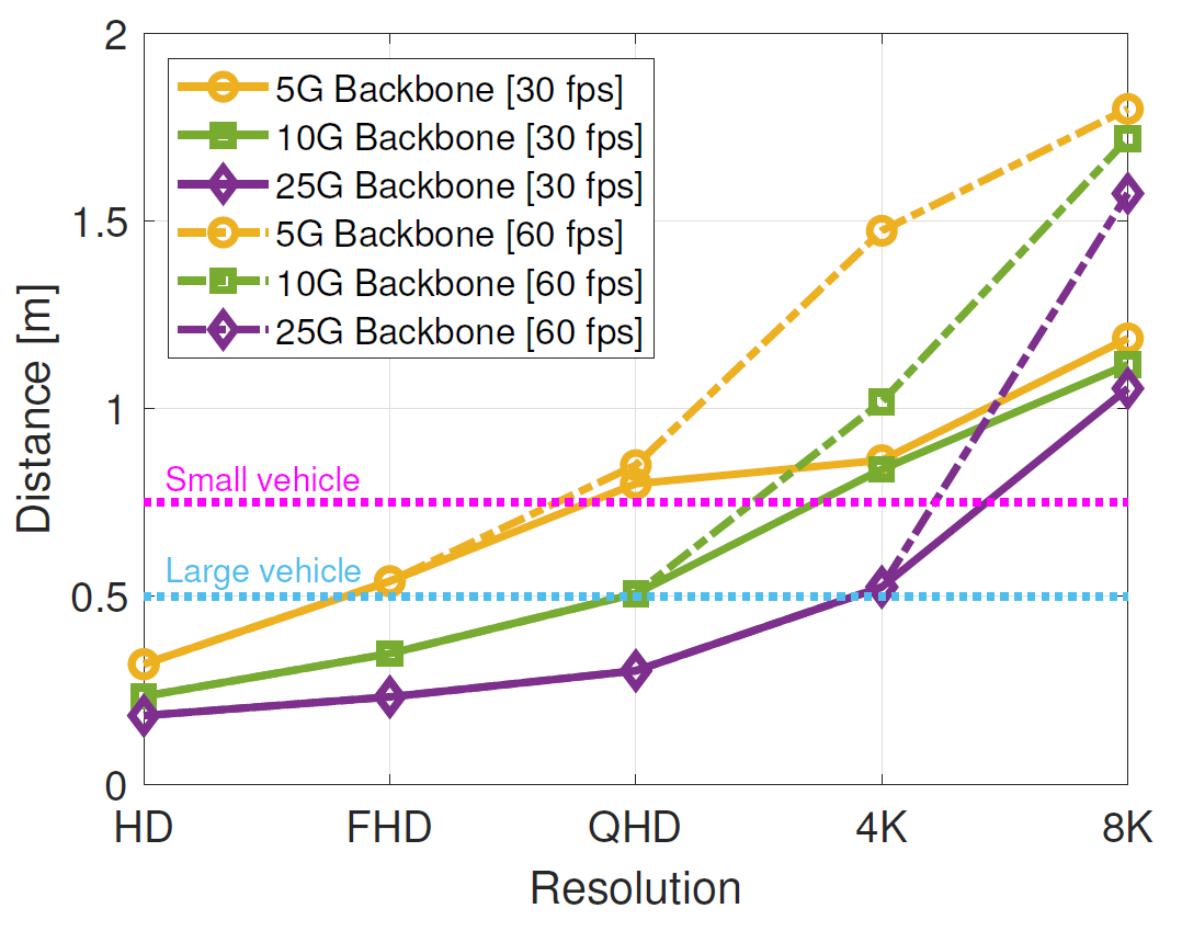
Taking the small vehicle as an example, [TeX:] $$e_d$$ of the vehicle with the HD camera resolution is lower than [TeX:] $$e_m$$ in all Ethernet backbones. [TeX:] $$e_d$$ of the vehicle with the FHD camera resolution is lower than [TeX:] $$e_m$$ in the 10G and 25G Ethernet backbones, but [TeX:] $$e_d$$ exceeds [TeX:] $$e_m$$ in the 5G Ethernet backbones. For the QHD resolution, [TeX:] $$e_d$$ of the vehicle is lower than [TeX:] $$e_m$$ only in the 25G case, and [TeX:] $$e_d$$ exceeds [TeX:] $$e_m$$ in all Ethernet backbones with resolutions of 4K and 8K, where we should consider additional data compression at the cost of additional computation.
The proper compression ratio to meet [TeX:] $$e_m$$ is shown in Fig. 8. Note that all the appropriate compression ratios are higher than the sensor period of 60 fps so that it can operate under both 30 fps and 60 fps sensor periods. The maximum compression ratio is set to 99.9%. The black boundary line indicates [TeX:] $$e_m$$, which is 0.5 m for a large vehicle and 0.75 m for a small vehicle. Each color of the domains indicates whether the vehicle can satisfy the lateral distance threshold or not. The red domain means [TeX:] $$e_d \geq 0.75$$, the orange domain means [TeX:] $$0.5 \leq e_d \leq 0.75$$, and the yellow domain means [TeX:] $$e_d \lt 0.5.$$ For example, a large vehicle satisfies the lateral distance threshold condition in the yellow domain, and a small vehicle meets the lateral distance threshold condition in both the yellow and orange domains. Taking the large vehicle with the 5G Ethernet backbone as an example, the resolution of HD can satisfy the lateral distance threshold condition without compression.
However, compression becomes essential starting from FHD. To have [TeX:] $$e_d \text{ lower than } e_m$$ at the FHD, QHD, and 4K resolutions, compression ratios of approximately 18%, 60%, and 92% as shown in Fig. 8(a), are required. However, even with compression of camera sensor data at 8K resolution, [TeX:] $$e_d \text{ exceeds } e_m,$$ making it unfeasible to support LKAS.
Fig. 8.
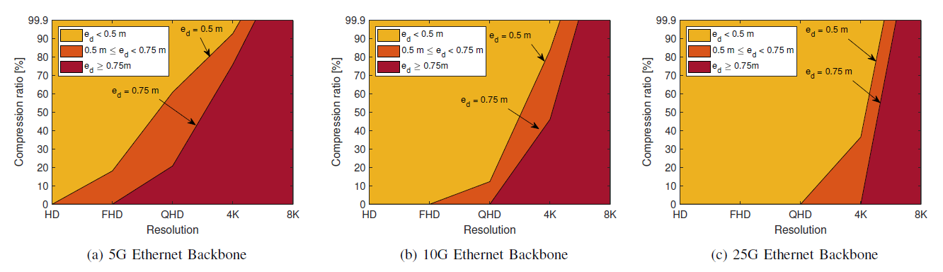
Table 4 shows the proper compression ratio and available longitudinal speed of each resolution to satisfy the lateral distance threshold condition. Here, the maximum speed of the vehicle is 19.001 m/s referring to the product of the maximum heading angle ([TeX:] $$20^{\circ}$$) and maximum vehicle speed (200 km/h). For a large vehicle, a vehicle with the 5G Ethernet backbone can only use HD cameras without data compression. Also, without compression, a large vehicle with the 10G backbone can use camera resolutions up to the FHD range, and a vehicle with the 25G backbone can use camera resolutions up to QHD. With data compression, a large vehicle can use camera resolutions up to 4K in all Ethernet backbones. However, 8K cameras cannot be used in large vehicles even with 99.9% data compression considering the maximum vehicle speed of 19.001 m/s.
TABLE IV
| Vehicle size | Resolution | Compression ratio for LKAS (%) | Available longitudinal speed (m/s) | ||||
|---|---|---|---|---|---|---|---|
| 5G | 10G | 25G | 5G | 10G | 25G | ||
| Large ([TeX:] $$e_m=0.5$$) | HD | 0 | 0 | 0 | 19.001 | 19.001 | 19.001 |
| FHD | 18.12 | 0 | 0 | 19.001 | 19.001 | 19.001 | |
| QHD | 60.86 | 12.3 | 0 | 19.001 | 19.001 | 19.001 | |
| 4K | 92.76 | 83.77 | 36.52 | 19.001 | 19.001 | 19.001 | |
| 8K | Impossible | Impossible | Impossible | 8.561 | 8.586 | 8.601 | |
| Small ([TeX:] $$e_m=0.75$$) | HD | 0 | 0 | 0 | 19.001 | 19.001 | 19.001 |
| FHD | 0 | 0 | 0 | 19.001 | 19.001 | 19.001 | |
| QHD | 20.81 | 0 | 0 | 19.001 | 19.001 | 19.001 | |
| 4K | 75.96 | 46.14 | 0 | 19.001 | 19.001 | 19.001 | |
| 8K | Impossible | Impossible | Impossible | 12.841 | 12.879 | 12.902 | |
A small vehicle with the 5G backbone can use camera resolutions up to the FHD range without data compression. Also, without compression, a small vehicle with the 10G backbone can use camera resolutions up to QHD, and a vehicle with the 25G backbone can use camera resolutions up to 4K. With data compression, large vehicles with 5G and 10G backbones can also use camera resolutions up to 4K. However, 8K camera cannot be used, as in small vehicles, even with 99.9% data compression considering the maximum vehicle speed of 19.001 m/s.
When a vehicle satisfies the lateral distance threshold, the available longitudinal speed is 19.001 m/s. However, for both vehicle types with 8K cameras, even when compressing the camera data to the maximum compression ratio, [TeX:] $$e_d$$ remains larger than [TeX:] $$e_m$$, preventing the vehicles from operating at maximum speed. The available longitudinal speed with the 8K camera is from 8.561 to 8.601 m/s for a large vehicle and from 12.841 to 12.902 m/s for a small vehicle when the compression ratio is 99.9%. Finally, it becomes possible to determine the proper resolutions and compression ratios with the Ethernet backbone for all vehicle types. In the designed vehicle architecture, vehicles with up to 4K cameras are able to satisfy the lateral distance threshold, with data compression. However, an increase in the data rate of the Ethernet backbone is required to use the 8K camera. This can be considered in the future standardization of higher-rate automotive Ethernet.
V. CONCLUSION
This paper focuses on analyzing the impact of IVN latency on LKAS. To assess the LKAS performance, we considered a lateral error distance and lateral distance threshold, taking into account the end-to-end latency. The study analyzed the factors contributing to end-to-end latency in an LKAS system, identifying IVN latency and processing latency as key factors. To evaluate the end-to-end latency, a next-generation IVN topology was designed, considering the zonal architecture with an Ethernet backbone. A system-level simulation of the IVN topology was conducted using OMNeT++ to validate the analysis results. To ensure data integrity, a required compression ratio was determined based on the camera’s sensor period and resolution. Subsequently, the end-to-end latency of the designed IVN topology with the required compression ratio was calculated. Based on the obtained end-to-end latency, the paper proposed lateral error distances for different vehicles. A graph was introduced to determine whether a vehicle equipped with cameras at various resolutions satisfies the lateral distance threshold condition or not. In cases where high-resolution cameras are impractical due to latency constraints, guidelines were provided to determine the required compression ratio for each resolution and the maximum longitudinal speed of the vehicle at that compression ratio. The queuing latency in this study was deemed negligible, as the network traffic load was relatively low, considering the single function of LKAS. However, it is acknowledged that queuing latency should be considered in more complex future vehicle networks that support diverse ADAS or autonomous vehicle functions with higher network traffic. Additionally, further validation of the simulation results in real-world vehicle testing environments is necessary. In the future, we plan to consider the resolution and quantity of various sensors, including LiDAR and radar, in addition to cameras, and apply technologies like 3D road lane classification with improved texture patterns and optimized deep classifier to our research. This will enable us to implement more realistic and diverse ADAS functions and analyze associated factors such as IVN latency. Through this analysis, we can enhance the efficiency and stability of autonomous vehicles when applied in realworld autonomous driving scenarios by using the optimal sensor combination that meets the latency requirements.
Biography
Sinuk Choi

Sinuk Choi received the B.S. degree in Electronics Engineering from Kyungpook National University, Daegu, South Korea, in 2017. He is currently pursuing the Ph.D. degree with the Department of Electrical Engineering and Computer Science, Daegu Gyeongbuk Institute of Science and Technology, Daegu, South Korea. His research interests include vehicle-to-everything communication, autonomous driving, and cellular communication system.
Biography
Hoseung Song

Hoseung Song received his M.S degree in the Department of Electrical Engineering and Computer Science from DGIST, Daegu, South Korea, in 2022, where he received a B.S degree in 2019. He is currently with AUTOCRYPT, Seoul, South Korea. His research interests include in-vehicle networks such as in-vehicle SerDes and automotive Ethernet.
Biography
Eunmin Choi
Eunmin Choi received the B.S. degree in Electronics Engineering from Kyungpook National University, Daegu, South Korea, in 2014. Since 2015, she has been with the Department of Electrical Engineering and Computer Science, DGIST, Daegu, South Korea, where she received a M.S. degree in 2017 and is currently working toward a Ph.D. degree. Her research interests include in-vehicle networks and vehicular security.
Biography
Biography
Ji-Woong Choi
Ji-Woong Choi (Senior Member, IEEE) received the B.S., M.S., and Ph.D. degrees from Seoul National University, Seoul, South Korea, in 1998, 2000, and 2004, respectively, all in Electrical Engineering. From 2004 to 2005, he was a Postdoctoral Researcher with the Inter-University Semiconductor Research Center, SNU. From 2005 to 2007, he was a Postdoctoral Visiting Scholar with the Department of Electrical Engineering, Stanford University, Stanford, CA, USA. He was also a Consultant with GCT Semiconductor, San Jose, CA, USA, for the development of mobile TV receivers, from 2006 to 2007. From 2007 to 2010, he was with Marvell Semiconductor, Santa Clara, CA, USA, as a Staff Systems Engineer for next-generation wireless communication systems, including WiMAX and LTE. Since 2010, he has been with the Department of Electrical Engineering and Computer Science, Daegu Gyeongbuk Institute of Science and Technology (DGIST), Daegu, South Korea, as a Professor. His research interests include wireless communication theory, signal processing, biomedical communication applications, and brain-machine interface.
References
- 1 A. Ouaknine, A. Newson, J. Rebut, F. Tupin, and P. Perez, "CARRADA dataset: Camera and automotive radar with range angle doppler annotations," in Proc. ICPR, 2021.doi:[[[10.48550/arXiv.2005.01456]]]
- 2 J.-S. Lee, K. Choi, T. Park, and S.-C. Kee, "A study on the vehicle detection and tracking using forward wide angle camera," Trans. Korean Soc. Automotive Engineers, vol. 26, no. 3, pp. 368-377, 2018.doi:[[[10.7467/KSAE.2018.26.3.368]]]
- 3 A. Aydt, "Advances towards a compact in-vehicle Ethernet, camera, radar & LIDAR measurement for high-bandwidth driver assistance systems." Vector, 2019. Accessed: Aug. 3, 2023. (Online). Available: https://cdn.vector.com/cms/content/events/2019/VH/VIC2019/5 Adva nces towards a compact in-vehicle Ethernet Camera Radar L IDAR .pdfcustom:[[[https://cdn.vector.com/cms/content/events/2019/VH/VIC2019/5Advancestowardsacompactin-vehicleEthernetCameraRadarLIDAR.pdf]]]
- 4 W. Zeng, M. A. S. Khalid, and S. Chowdhury, "In-vehicle networks outlook: Achievements and challenges," IEEE Commun. Surveys Tuts., vol. 18, no. 3, pp. 1552-1571, 2016.doi:[[[10.1109/COMST.2016.2521642]]]
- 5 H. Zinner, "Automotive Ethernet and SerDes in competition," ATZ electronics worldwide, vol. 15, no. 7, pp. 40-43, 2020.doi:[[[10.1007/s38314-020-0232-0]]]
- 6 Greater than 10 Gb/s electrical automotive Ethernet task force, IEEE P802.3cy, 2021.custom:[[[-]]]
- 7 A. Frigerio, B. Vermeulen, and K. G. W. Goossens, "Automotive architecture topologies: Analysis for safety-critical autonomous vehicle applications," IEEE Access, vol. 9, pp. 62837-62846, 2021.doi:[[[10.1109/ACCESS.2021.3074813]]]
- 8 O. Alparslan, S. Arakawa, and M. Murata, "Next generation intravehicle backbone network architectures," in Proc. IEEE HPSR, 2021.doi:[[[10.1109/HPSR52026.2021.9481803]]]
- 9 V . Bandur, G. Selim, V . Pantelic, and M. Lawford, "Making the case for centralized automotive E/E architectures," IEEE Trans. Veh. Technol., vol. 70, no. 2, pp. 1230-1245, 2021.doi:[[[10.1109/TVT.2021.3054934]]]
- 10 H.-J. Cha, W.-H. Jeong, and J.-C. Kim, "Control-scheduling codesign exploiting trade-off between task periods and deadlines," Mobile Information Systems, vol. 2016, pp. 1-11, 2016.doi:[[[10.1155/2016/3414816]]]
- 11 T. Tanaka, S. Nakajima, T. Urabe, and H. Tanaka, "Development of lane keeping assist system using lateral-position-error control at forward gaze point," tech. rep., SAE Technical Paper, 2016. Accessed: Sep. 18, 2023. (Online). Available: https://www.sae.org/publications/technicalpapers/content/2016-01-0116/custom:[[[https://www.sae.org/publications/technicalpapers/content/2016-01-0116/]]]
- 12 H. Liu, C. Liu, L. Hao, and D. Zhang, "Stability analysis of lane-keeping assistance system for trucks under crosswind conditions," Applied Sciences, vol. 13, no. 17, 2023.doi:[[[10.3390/app13179891]]]
- 13 S. Wei, P. E. Pfeffer, and J. Edelmann, "State of the art: Ongoing research in assessment methods for lane keeping assistance systems," IEEE Trans. Intell. Veh., pp. 1-28, 2023.doi:[[[10.1109/TIV.2023.3269156]]]
- 14 Y . Liu and H. Zhang, "Robust driver-automation shared control for a lane keeping system using interval type 2 fuzzy method," in Proc. IEEE ISIE, 2019.doi:[[[10.1109/ISIE.2019.8781342]]]
- 15 X. Zhou, H. Shen, Z. Wang, H. Ahn, and J. Wang, "Driver-centric lane-keeping assistance system sesign: A noncertainty-equivalent neuroadaptive control approach," IEEE/ASME Trans. Mechatronics, pp. 1-12, 2023.doi:[[[10.1109/TMECH.2023.3236245]]]
- 16 B. Janakiraman, S. Shanmugam, R. P´ erez de Prado, and M. Wozniak, "3D road lane classification with improved texture patterns and optimized deep classifier," Sensors, vol. 23, no. 11, 2023.doi:[[[10.3390/s23115358]]]
- 17 I. Goel, "Simulation-based end-to-end latency analysis of ADAS systems," Master’s thesis, Dept. Elect. Eng., Delft Univ. of Tech., Delft, Netherlands, 2018.custom:[[[-]]]
- 18 D. H. Kim, N. Young Lee, J. M. Rhee, and S. Yoon Park, "Performance analysis for HSR based in-vehicular network (IVN) under end-to-end latency (EEL) constraint with store-and-forward mode," in Proc. ICTC, 2020.doi:[[[10.1109/ICTC49870.2020.9289606]]]
- 19 D.-Y . Kim, M. Jung, and S. Kim, "An Internet of vehicles (IoV) access gateway design considering the efficiency of the in-vehicle Ethernet backbone," Sensors, vol. 21, no. 1, 2021.doi:[[[10.3390/s21010098]]]
- 20 Z. Zhou, J. Lee, M. S. Berger, S. Park, and Y . Yan, "Simulating TSN traffic scheduling and shaping for future automotive Ethernet," J. Commun. Netw., vol. 23, no. 1, pp. 53-62, 2021.doi:[[[10.23919/JCN.2021.000001]]]
- 21 H. Kim, W. Yoo, S. Ha, and J.-M. Chung, "In-vehicle network average response time analysis for CAN-FD and automotive Ethernet," IEEE Trans. Veh. Technol., vol. 72, no. 6, pp. 6916-6932, 2023.doi:[[[10.1109/TVT.2023.3236593]]]
- 22 M. Reke et al., "A self-driving car architecture in ROS2," in Proc. SAUPEC/RobMech/PRASA, 2020.doi:[[[10.1109/SAUPEC/RobMech/PRASA48453.2020.9041020]]]
- 23 B. Purvis, "Honda motorcycle lane keep assist." Cycle world, 2022. Accessed: Oct. 24, 2023. (Online). Available: https://www.cycleworld.com/story/motorcycle-news/honda-developingmotorcycle-lane-keep-assist/custom:[[[https://www.cycleworld.com/story/motorcycle-news/honda-developingmotorcycle-lane-keep-assist/]]]
- 24 "Lane keeping assist system (LKAS)." Honda Info Center, 2022. Accessed: Oct. 24, 2023. (Online). Available: https://www.hondainfocenter.com/2022/Passport/FeatureGuide/Interior-Features/Lane-Keeping-Assist-System/custom:[[[https://www.hondainfocenter.com/2022/Passport/FeatureGuide/Interior-Features/Lane-Keeping-Assist-System/]]]
- 25 Rules for road structure and facilities standards, Minister of Land, Infrastructure, and Transport, 2021.custom:[[[-]]]
- 26 Hyundai, "SANTA FE specifications ," 2019. Accessed: Aug. 3, 2023. (Online). Available: https://www.hyundai.com/kr/ko/e/vehicles/santafe/speccustom:[[[https://www.hyundai.com/kr/ko/e/vehicles/santafe/spec]]]
- 27 Hyundai, "XCIENT specification ," 2015. Accessed: Aug. 3, 2023. (Online). Available: http://trucknbus.hyundai.com/global/products/truck/xcientcustom:[[[http://trucknbus.hyundai.com/global/products/truck/xcient]]]
- 28 A. D. Santos et al., "Characterization of substation process bus network delays," IEEE Trans. Ind. Informat., vol. 14, no. 5, pp. 2085-2094, 2018.doi:[[[10.1109/TII.2017.2731618]]]
- 29 Y . Lee, J. Kim, and J. Jeon, "Automotive diagnostic gateway using diagnostic over Internet protocol," IEIE Trans. Smart Process. Comput., vol. 3, no. 5, pp. 313-318, 2014.doi:[[[10.5573/IEIESPC.2014.3.5.313]]]
- 30 H. Choi, J. Choi, and Y . Jang, "Numerical analysis of queuing delay in cyclic bandwidth allocation TDMA system," Electronics Letters, vol. 50, no. 17, pp. 1204-1205, 2014.doi:[[[10.1049/el.2014.0351]]]
- 31 S. De et al., "Approximation trade offs in an image-based control system," in Proc. DATE, 2020.doi:[[[10.23919/DATE48585.2020.9116552]]]
- 32 A. Howard et al., "Searching for mobileNetV3," in Proc. IEEE/CVF ICCV, 2019.doi:[[[10.48550/arXiv.1905.02244]]]
- 33 R. M. Schreier and A. Rothermel, "A latency analysis on H.264 video transmission systems," in Proc. IEEE ICCE, 2008.doi:[[[10.1109/ICCE.2008.4588001]]]
- 34 I. Rozas-Ramallal, T. M. Fern´ andez-Caram´ es, A. Dapena, and J. A. Garc´ ıa-Naya, "Evaluation of H.264/A VC over IEEE 802.11p vehicular networks," EURASIP J. Advances Signal Process., vol. 2013, no. 1, pp. 1-13, 2013.doi:[[[10.1186/1687-6180-2013-77]]]
- 35 Y .-H. Chen and V . Sze, "A deeply pipelined CABAC decoder for HEVC supporting level 6.2 high-tier applications," IEEE Trans. Circuits Syst. Video Technol., vol. 25, no. 5, pp. 856-868, 2014.doi:[[[10.1109/TCSVT.2014.2363748]]]
- 36 "All Tesla cars being produced now have full self-driving hardware." Tesla, 2016. Accessed: Oct. 24, 2023. (Online). Available: https://www.tesla.com/blog/all-tesla-cars-being-produced-nowhave-full-self-driving-hardwarecustom:[[[https://www.tesla.com/blog/all-tesla-cars-being-produced-nowhave-full-self-driving-hardware]]]
- 37 "How many cameras do Tesla’s have?." Pimp My EV, 2022. Accessed: Oct. 24, 2023. (Online). Available: https://pimpmyev.com/blogs/speedstyle-carbon-fiber/how-many-cameras-do-teslas-havecustom:[[[https://pimpmyev.com/blogs/speedstyle-carbon-fiber/how-many-cameras-do-teslas-have]]]
- 38 M. Merano, "Tesla semi 10-camera setup observed in production autopilot code." Teslarati, 2020. Accessed: Oct. 24, 2023. (Online). Available: https://www.teslarati.com/tesla-semi-productioncamera-setup-revealed/custom:[[[https://www.teslarati.com/tesla-semi-productioncamera-setup-revealed/]]]
- 39 IEEE standard for local and metropolitan area network bridges and bridged networks, IEEE 802.1Q, 2018.custom:[[[-]]]
- 40] K. Neuenhueskes, "Integration of superior SoC solutions into zonal automotive networks." Toshiba, 2022. Accessed: Sep. 19, 2023. [Online Integration of superior SoC solutions into zonal automotive networks." Toshiba, 2022. Accessed: Sep. 19, 2023. [Online-sciedit-2-03"> K. Neuenhueskes, "Integration of superior SoC solutions into zonal automotive networks." Toshiba, 2022. Accessed: Sep. 19, 2023. [Online]. Available: https://www.allaboutcircuits.com/news/with-new-phytransceivers-microchip-progresses-automotive-ethernet/ K. Neuenhueskes, Toshiba, 2022. Accessed: Sep. 19, 2023. [Online]. Available: , https://www.allaboutcircuits.com/news/with-new-phytransceivers-microchip-progresses-automotive-ethernet/ , custom:[[[, https://www.allaboutcircuits.com/news/with-new-phytransceivers-microchip-progresses-automotive-ethernet/ , ]]].
- 41 Y . Onuma, Y . Terashima, and R. Kiyohara, "ECU software updating in future vehicle networks," in Proc. WAINA, 2017.doi:[[[10.1109/WAINA.2017.45]]]
- 42 T. Steinbach et al., "Beware of the hidden! how cross-traffic affects quality assurances of competing real-time Ethernet standards for in-car communication," in Proc. LCN, 2015.doi:[[[10.1109/LCN.2015.7366277]]]