State-Dependent Broadcast Channels with Reversible Input Constraints

I. INTRODUCTION

COMMUNICATION over channels whose transition probability depends upon an external state process have long been studied [1]–[5]. Much attention has been dedicated in the literature to the case of independent and identically distributed (i.i.d.) states that are available at either the encoder or the decoder, or both. State-dependent channels have also been investigated in multi-terminal settings, see for instance the broadcast model in [6]. The reader is referred to the survey work [7] for a comprehensive overview of channel coding problems in the presence of state information.

In a state-dependent communication system, the decoder is often interested in reconstructing certain information embedded in the transmission, in addition to reliably recovering the source message. Sutivong et al. [8], for example, considered a simultaneous message transmission and channel state amplification problem. They provided a complete characterisation of the optimal tradeoff between message transmission rate and state information reconstruction distortion over the Gaussian dirty paper channel [9] as assessed by mean-squared error measure. Kim et al. [10] then extended this problem from the Gaussian to the general discrete-memoryless scenario, with state information reconstruction fidelity evaluated by a list-size uncertainty reduction metric. Choudhuri et al. [11] subsequently analyzed the casual discrete-memoryless case with a general distortion metric. A multi-user extension of state estimation in a Gaussian multiple-access scenario was addressed in [12], wherein a complete characterization of the optimal rate-distortion trade-off region was obtained. This state information reconstruction problem sparked extensive research on other information reconstruction problems such as state masking [13], [14], partial/remote state estimation [15], [16], common reconstruction [17], [18], and information embedding motivated by Witsenhausen’s counterexample [19], [20].

Communication systems with constrained inputs have been studied in various contexts. For instance, Sumszyk and Steinberg [21] focused on lossless input reconstruction over a statedependent single-user channel in an information embedding context. Bandemer and El Gamal [22] discussed a setting where the amount of disturbance caused to other users by a given transmission must be minimized. Zhang et al. [23] investigated channel coding subject to signal estimation constraints in the absence of state information at the encoder. However, we note that multi-terminal settings with communication and input reconstruction constraints have received scant attention in the literature, which is of interest in several applications, as described below.

In this study, we address a communication problem over a discrete-memoryless state-dependent degraded broadcast channel with an input reconstruction constraint at the degraded receiver, with noncausal state information at the transmitter and the non-degraded receiver. This is of interest, for instance in watermarking systems [24], where the encoder must encode messages to two receivers, one of which has access to the covertext (which corresponds to the state process), while the other receiver must be able to reproduce the stegotext (which corresponds to the channel input codeword) for retransmission to another destination. For this problem, we explore and characterize the optimal tradeoff between reliable communication rates and reconstruction distortion using a general distortion measure. Our bounds also yield a tight result for a binary broadcast channel with Hamming distortion. The achievability proof relies on adapting the approach for state-dependent broadcast channels from [6], while the outer bound relies on appropriate auxiliary identifications to manipulate the noni. i.d. channel input sequence. Compared to a joint sourcechannel coding problem (see for instance [25, Chapter 3]) which usually involves transmission of an i.i.d. source over a given channel in a lossy/lossless manner, the problem addressed in this paper instead involves an estimation of the message-bearing non-i.i.d. channel input codeword at the receiver. The term ‘reversible input constraints’ is used in this context to refer to such recovery of the input from an observation of the channel output sequence

The rest of the paper is organized as follows. The system model and main result (Theorem. 1) are introduced in Section II. Section III contains the proof of achievability for Theorem. 1 while its converse is proved in Section IV. A tight characterization is worked out for the binary additive broadcast channel in Section V. Concluding remarks are given in Section VI.

Notations: Random variables/vectors are denoted by uppercase letters, while their realizations are denoted by the corresponding lower case letters. A sequence [TeX:] $$\left(X_1, X_2, \cdots, X_n\right)$$ is denoted by [TeX:] $$X^n$$ for convenience.

II. SYSTEM MODEL AND RESULTS

Consider the system shown in Fig. 1. Let [TeX:] $$\mathcal{X}, \mathcal{S}, \mathcal{Y}_1, \mathcal{Y}_2, \hat{\mathcal{X}}$$ be finite sets, and [TeX:] $$p_S(s)$$ be a probability mass function on [TeX:] $$\mathcal{S}.$$ The given system is that of a discrete-memoryless broadcast channel (DM-BC) with discrete memoryless states, denoted by the tuple [TeX:] $$\left(\mathcal{S}, p_S(s), \mathcal{X}, p_{Y_1, Y_2 \mid X, S}\left(y_1, y_2 \mid x, s\right), \mathcal{Y}_1, \mathcal{Y}_2\right) .$$ The channel is characterized by an input alphabet [TeX:] $$\mathcal{X}$$, state alphabet [TeX:] $$\mathcal{S}$$, output alphabet [TeX:] $$\mathcal{Y}_1 \times \mathcal{Y}_2,$$ and conditional probability mass function [TeX:] $$p_{Y_1, Y_2 \mid X, S}\left(y_1, y_2 \mid x, s\right).$$ The channel and the states are assumed to be memoryless, i.e.,

We assume that the channel is degraded, i.e.,

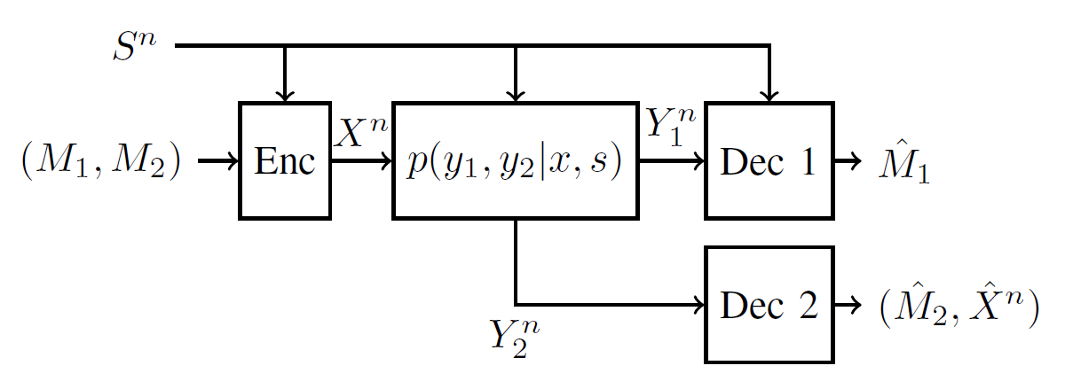
The channel state is assumed to be known non-causally to the transmitter as well as the non-degraded receiver [TeX:] $$Y_1$$ (also referred to as the strong receiver), while the degraded receiver [TeX:] $$Y_2$$ (also known as the weak receiver) is uninformed. We wish to communicate messages [TeX:] $$\left(M_1, M_2\right)$$ over the channel, and at the same time also reconstruct the input codeword at the weak receiver (depicted [TeX:] $$\hat{X}^n$$ in Fig. 1) to meet a distortion constraint. The distortion measure is defined as

where [TeX:] $$\hat{\mathcal{X}}$$ is the reconstruction alphabet.

Definition 1. An [TeX:] $$\left(n, 2^{n R_1}, 2^{n R_2}\right)$$ code consists of two message sets [TeX:] $$\left\{1,2, \cdots, 2^{n R_j}\right\}, j \in\{1,2\}$$ on which [TeX:] $$M_j$$ are assumed to be uniformly distributed, an encoder map that assigns a codeword [TeX:] $$x^n \in \mathcal{X}^n$$ to each [TeX:] $$m_j \in\left\{1,2, \cdots, 2^{n R_j}\right\}, j \in \{1,2\} \text { and } s^n \in \mathcal{S}^n \text {, }$$ a decoder map at the strong receiver that assigns an estimate [TeX:] $$\hat{m}_1 \in\left\{1,2, \cdots, 2^{n R_1}\right\}$$ to each received sequence [TeX:] $$\left(y_1^n, s^n\right) \in \mathcal{Y}_1^n \times \mathcal{S}^n,$$ and a decoder map at the weak receiver that assigns a pair of estimates [TeX:] $$\left(\hat{m}_2, \hat{x}^n\right) \in\left\{1,2, \cdots, 2^{n R_2}\right\} \times \hat{\mathcal{X}}^n$$ to each received sequence [TeX:] $$y_2^n \in \mathcal{Y}_2^n .$$ The average probability of error is given by

A rate-distortion triple [TeX:] $$\left(R_1, R_2, D\right)$$ is said to be achievable if there exists a sequence of [TeX:] $$\left(n, 2^{n R_1}, 2^{n R_2}\right)$$ codes such that

and

The rate-distortion trade-off region [TeX:] $$\mathcal{C}$$ is the closure of the set of all achievable [TeX:] $$\left(R_1, R_2, D\right)$$ triples. The main result of this paper is stated next.

Theorem 1. The rate-distortion trade-off region [TeX:] $$\mathcal{C}$$ for the degraded DM-BC with non-causal state information known to the encoder as well as the strong receiver, and input reconstruction constraints at the weak receiver, is the closure of the set that contains all triples [TeX:] $$\left(R_1, R_2, D\right)$$ that satisfy

for some joint probability distribution of the form

and some function [TeX:] $$\phi: \mathcal{U} \times \mathcal{Y}_2 \rightarrow \hat{\mathcal{X}},$$ with the auxiliary random variable cardinality bounded as [TeX:] $$|\mathcal{U}| \leq|\mathcal{X}| \cdot|\mathcal{S}|+2 .$$

Proof. The achievability is proved in Section III, while the converse proof is given in Section IV.

We note that expression (6) also appears in the capacity of a state-dependent single-user channel with non-causal state information at the transmitter [3]. Expression (7) also appears as the rate constraint for the strong receiver in a degraded statedependent broadcast channel [6]. However, the key difference in this paper compared to known works is the addition of constraint (8) in our region that takes care of the codeword distortion tolerance requirement.

Remark 1. The definition in (1) corresponds to a physically degraded broadcast channel, i.e. [TeX:] $$(X, S) \rightarrow Y_1 \rightarrow Y_2$$ is a Markov chain. On the other hand, the broadcast channel is said to be stochastically degraded if there exists [TeX:] $$\tilde{Y}_1$$ such that [TeX:] $$\tilde{Y}_1 \mid\{X=x, S=s\} \sim p_{Y_1 \mid X, S}\left(\tilde{y}_1 \mid x, s\right),$$ i.e. [TeX:] $$\tilde{Y}_1$$ has the same conditional pmf as [TeX:] $$Y_1$$ given [TeX:] $$(X, S), \text{ and }(X, S) \rightarrow Y_1 \rightarrow Y_2$$ is a Markov chain (see also [25, Chapter 5]).

As far as the probability of error requirement (4) is concerned, since the capacity region of the broadcast channel [TeX:] $$p_{Y_1, Y_2 \mid X, S}\left(y_1, y_2 \mid x, s\right)$$ depends only upon the marginal distributions [TeX:] $$p_{Y_1 \mid X, S}\left(y_1 \mid x, s\right)$$ and [TeX:] $$p_{Y_2 \mid X, S}\left(y_2 \mid x, s\right),$$ no distinction needs to be made between physical and stochastic degradation. Furthermore, notice that the distortion requirement (5) depends only upon the marginal distribution of [TeX:] $$Y_2$$, i.e. [TeX:] $$p_{Y_2 \mid X, S}\left(y_2 \mid x, s\right),$$ and not on the marginal distribution of [TeX:] $$Y_1$$. This is because the input reconstruction [TeX:] $$\hat{X}^n$$ and the corresponding expected distortion [TeX:] $$\mathbb{E}\left[d\left(X^n, \hat{X}^n\right)\right]$$ depend only upon the degraded output [TeX:] $$Y_2^n,$$ and not on the non-degraded output [TeX:] $$Y_1^n.$$ Hence, even with respect to the distortion requirement, no distinction needs to be made between physical and stochastic degradation. Therefore, the proofs in the sequel go through even if the broadcast channel is stochastically degraded, and henceforth we shall simply refer to the broadcast channel as being degraded.

III. ACHIEVABILITY PROOF OF THEOREM 1

The achievability is proven using a combination of Gelfand- Pinsker coding and superposition coding. Here, a U codebook is built first which shall be a compression codebook for the state sequence and is binned according to the weak user’s message. Then for each [TeX:] $$u^n$$ sequence, a conditional codebook shall be generated according to the strong user’s message. We denote the set of jointly −typical n−length sequences with respect to a joint distribution [TeX:] $$p_{A, B}(a, b)$$ by [TeX:] $$\mathcal{T}_\epsilon^n(A, B),$$ as in [25]. Fix the pmf [TeX:] $$p(u \mid s) p(x \mid u, s)$$ and function [TeX:] $$\phi\left(u, y_2\right) .$$

Codebook generation:

Randomly and independently generate [TeX:] $$2^{n\left(R_2+R_2^{\prime}\right)}$$ sequences [TeX:] $$u^n\left(m_2, j_2\right), m_2 \in\left[1: 2^{n R_2}\right]$$ and [TeX:] $$j_2 \in\left[1: 2^{n R_2^{\prime}}\right]$$ i.i.d. according to [TeX:] $$\prod_{i=1}^n p_U\left(u_i\right)$$ and divide them into [TeX:] $$2^{n R_2}$$ bins [TeX:] $$\mathcal{B}_U\left(m_2\right) \text { for } m_2 \in\left[1: 2^{n R_2}\right] \text {. }$$ For each [TeX:] $$2^{n R_2}$$ sequence, randomly and conditionally independently generate [TeX:] $$2^{n R_1}$$ sequences [TeX:] $$x^n\left(m_2, j_2, m_1\right) \text { for } m_1 \in\left[1: 2^{n R_1}\right]$$ i.i.d. according to [TeX:] $$\prod_{i=1}^n p_{X \mid U}\left(x_i \mid u_i\right) .$$

Encoding:

Firstly, given [TeX:] $$m_2 \in\left[1: 2^{n R_2}\right] \text { and } s^n \text {, }$$ find a sequence [TeX:] $$u^n\left(m_2, j_2\right) \text { with } j_2 \in \mathcal{B}_U\left(m_2\right)$$ such that [TeX:] $$\left(u^n\left(m_2, j_2\right), s^n\right) \in \mathcal{T}_{\epsilon^{\prime}}^n(U, S) .$$ Declare error if no such index is found. Given [TeX:] $$m_1 \in\left[1: 2^{n R_1}\right] \text {, }$$ pick the sequence [TeX:] $$x^n\left(m_2, j_2, m_1\right)$$ in the conditional codebook corresponding to the chosen [TeX:] $$u^n\left(m_2, j_2\right)$$ sequence, which is then transmitted over the channel.

Decoding:

Let [TeX:] $$\epsilon \gt \epsilon^{\prime} .$$ The weak receiver declares that [TeX:] $$\hat{m}_2$$ is sent if it is the unique message such that [TeX:] $$\left(u^n\left(\hat{m}_2, \hat{j}_2\right), y_2^n\right) \in \mathcal{T}_\epsilon^n\left(U, Y_2\right)$$ for some [TeX:] $$\hat{j}_2 \in \mathcal{B}_U\left(\hat{m}_2\right) .$$ Declare error if no such message is found or if more than one are found. At the strong user, we use simultaneous decoding [25, eq. (6.3)]. The strong user declares that [TeX:] $$\hat{m}_1$$ is sent if it is the unique message such that [TeX:] $$\left(u^n\left(\hat{m}_2, \hat{j}_2\right), s^n, x^n\left(\hat{m}_2, \hat{j}_2, \hat{m}_1\right), y_1^n\right) \in \mathcal{T}_\epsilon^n\left(U, X, S, Y_1\right)$$ for some [TeX:] $$\hat{m}_2 \text { and } \hat{j}_2 \in \mathcal{B}_U\left(\hat{m}_2\right) \text {. }$$ Declare error if no such message is found or if more than one are found.

Analysis of probability of error:

Assume without loss of generality that the messages [TeX:] $$M_1=1$$ and [TeX:] $$M_2=1$$ were sent, and the index of the chosen [TeX:] $$U^n$$ sequence for [TeX:] $$M_1=1, M_2=1$$ and [TeX:] $$S^n \text{ and } J_2.$$ The encoding error events are as follows:

The decoding error events at the receivers are as follows:

The overall error event [TeX:] $$\mathcal{E}$$ is the union of the five error events listed above. By the union bound, we have:

By the covering lemma [25], the probability of encoding errors goes to zero as [TeX:] $$n \rightarrow \infty$$ as follows:

where [TeX:] $$\delta^{\prime}\left(\epsilon^{\prime}\right) \rightarrow 0 \text { as } \epsilon^{\prime} \rightarrow 0 .$$ By the packing lemma [25], the probability of decoding errors goes to zero as [TeX:] $$n \rightarrow \infty$$ as follows:

where [TeX:] $$\delta(\epsilon) \rightarrow 0 \text { as } \epsilon \rightarrow 0 \text {. }$$ However, we note that the constraint (18) follows from (16) and (17), and thus rendered inoperative due to the degraded nature of the channel. This can be seen as follows, by adding together (16) and (17):

where (a) follows from the degraded nature of the channel. Putting together equations (15) through (17), we arrive at the rate constraints:

Distortion analysis:

The mentioned distortion can be obtained by making the input estimate at the weak receiver on a per-letter basis. Since the function [TeX:] $$\phi\left(U, Y_2\right)$$ satisfies the distortion constraint, it follows from the random codebook construction that as [TeX:] $$n \rightarrow \infty,$$ we have

Thus the achievable region is proved.

IV. CONVERSE PROOF OF THEOREM 1

Given an achievable triple [TeX:] $$\left(R_1, R_2, D\right),$$ we need to prove that there exists a joint distribution of the form [TeX:] $$P_S P_{U \mid S} P_{X \mid U, S} P_{Y_1 \mid X, S} P_{Y_2 \mid Y_1}$$ and a function [TeX:] $$\phi(\cdot),$$ such that the rate-distortion constraints in Theorem 1 hold. To bound the weak user’s rate, consider the following chain of inequalities:

where (a) follows from Fano’s inequality with [TeX:] $$\epsilon_n \rightarrow 0$$ as [TeX:] $$n \rightarrow \infty$$ and since [TeX:] $$M_2$$ is independent of [TeX:] $$S^n,$$ (b) follows since the state process is i.i.d., (c) follows from the Csiszar-sum identity, while (d) follows with an auxiliary identification of [TeX:] $$U_i=\left(M_2, Y_2^{i-1}, S_{i+1}^n\right) .$$ Thus, we obtain

where (a) follows by introducing a time-sharing random variable Q uniform on [1, 2, . . . , n] that is independent of everything else, (b) follows since [TeX:] $$S_Q$$ is independent of Q and (c) follows by defining [TeX:] $$U=\left(Q, U_Q\right), X=X_Q, S=S_Q, Y_1=Y_{1,Q}$$ and [TeX:] $$Y_2=Y_{2,Q}.$$ Taking limits as [TeX:] $$n \rightarrow \infty$$ which makes [TeX:] $$\epsilon_n \rightarrow 0$$ completes the bound. Next, to bound the strong user’s rate, consider the following chain of inequalities:

where (a) follows since [TeX:] $$M_1$$ is independent of [TeX:] $$\left(M_2, S^n\right),$$ (b) follows from Fano’s inequality, (c) follows since [TeX:] $$X^n$$ is completely determined by [TeX:] $$\left(M_1, M_2, S^n\right),$$ (d) follows from the degraded nature of the broadcast channel, (e) follows from the memorylessness of the channel, while (f) follows from the earlier identification of [TeX:] $$U_i=\left(M_2, Y_2^{i-1}, S_{i+1}^n\right) .$$ Thus,

We next verify the expected distortion. By the distortion constraint in assumption, we have

where (a) follows by taking [TeX:] $$\phi_i\left(U_i, Y_{2 i}\right)=\hat{X}_i,$$ (b) follows by defining [TeX:] $$\phi:\left(Q, U_Q\right) \mapsto \phi_Q\left(U_Q\right)$$ and (c) follows since [TeX:] $$\left(U_Q, Q\right)=U, X_Q=X, \text { and } Y_{2, Q}=Y_2.$$ Finally, the bound on the auxiliary random variable cardinality [TeX:] $$|\mathcal{U}|$$ follows using the support lemma [25, Appendix C], as detailed in Appendix A. The converse proof is complete.

V. BINARY ADDITIVE BROADCAST CHANNEL WITH REVERSIBLE INPUTS

Suppose the input, state and reconstruction alphabets are restricted to be binary, i.e., [TeX:] $$\mathcal{X}=\mathcal{S}=\hat{\mathcal{X}}=\{0,1\} .$$ For the second receiver’s link, we consider an additive binary channel given by

where ⊕ denotes modulo-two addition, while the state S is a Bernoulli random variable independent of everything else, i.e., [TeX:] $$S \sim \operatorname{Ber}(p), p \in[0,1 / 2] .$$ Here, [TeX:] $$N_2$$ is another Bernoulli random variable specified by [TeX:] $$N_2 \sim \operatorname{Ber}\left(q_2\right), q_2 \in[0,1 / 2]$$ On the other hand, the first receiver’s link is another binary additive channel specified by

where [TeX:] $$N_1$$ is independent of everything else and is Bernoulli distributed, i.e., [TeX:] $$N_1 \sim \operatorname{Ber}\left(q_1\right), q_1 \in[0,1 / 2]$$ with [TeX:] $$q_1\lt q_2.$$ Notice that we can express

where [TeX:] $$\tilde{N} \sim \operatorname{Ber}(\tilde{q}) \text { and } q_2=q_1 * \tilde{q} \text {. }$$ At the weak receiver, the reconstruction distortion is defined in terms of the Hamming measure

We have the following theorem.

Theorem 2. For the input reconstruction problem over the given binary additive broadcast channel, the rate-distortion trade-off region is the closure of the set that contains all triples [TeX:] $$\left(R_1, R_2, D\right)$$ that satisfy

for some [TeX:] $$\alpha \in[0,1 / 2] \text {, with } H_2(a)=-a \log _2 a-(1-\text { a }) \log _2(1-a)$$ being the binary entropy function and [TeX:] $$a * b=a(1-b)+b(1-a)$$ denoting binary convolution.

Proof. The proof is based on an evaluation of the bounds in Theorem 1 for the given channel model. This is given in the following two subsections. The achievability is based on splitting the information transmission into two parts, one of which is for reliable communication while the other is intended for lossy input compression.

A. Proof of achievability for the binary broadcast channel

Choose independent random variables [TeX:] $$\left(U^{\prime}, \tilde{S}\right)$$ such that [TeX:] $$U^{\prime} \sim \operatorname{Ber}(1 / 2) \text { and } \tilde{S} \sim \operatorname{Ber}\left(\left(p-\left(D * q_2\right)\right) /\left(1-2\left(D * q_2\right)\right)\right) \text {. }$$ The joint distribution of [TeX:] $$(S, \tilde{S})$$ is such that [TeX:] $$\tilde{S}$$ is an input to a binary symmetric channel with crossover probability [TeX:] $$D * q_2,$$ and S is the corresponding output distributed as [TeX:] $$S \sim \operatorname{Ber}(p) .$$ In other words, we have

where [TeX:] $$N^{\prime} \sim \operatorname{Ber}(D)$$ is independent of everything else.

We now construct the auxiliary random variable U, the channel input X and the input codeword estimate at the weak receiver as

where [TeX:] $$N_2^{\prime} \sim \operatorname{Ber}(\alpha)$$ is independent of [TeX:] $$\left(U^{\prime}, S, N^{\prime}\right).$$ We now evaluate the mutual information terms in Theorem 1. The achievable rate for the weak user is

The achievable rate for the strong user is

The distortion constraint can be verified as follows:

This completes the proof of achievability.

B. Proof of converse for the binary broadcast channel

The converse proof involves invoking the single-letter expressions in Theorem 1. For the weak user’s rate, we have

where (a) follows since the estimate [TeX:] $$\hat{X}$$ is determined by [TeX:] $$\left(U, Y_2\right)$$ (b) follows since [TeX:] $$Y_2$$ is binary, while (c) follows since [TeX:] $$\operatorname{Pr}(X \neq \hat{X}) \leq D$$ and by invoking the monotonicity of the binary entropy function [TeX:] $$H_2(\cdot) \text { on }[0, p] \text {. }$$ For the strong user’s rate, we have

Since the following holds

there exists [TeX:] $$\alpha \in[0,1 / 2]$$ such that

Substituting (43) in (40), we obtain

Now let [TeX:] $$0 \leq H^{-1}(\nu) \leq 1 / 2$$ be the inverse of the binary entropy function. By the degraded nature of the channel and applying Mrs. Gerber’s lemma [25]

where [TeX:] $$\tilde{N} \text { and } \tilde{q}$$ are as in (29). This implies that

Substituting (46) in (41), we obtain

This completes the proof of converse.

C. Numerical Illustration

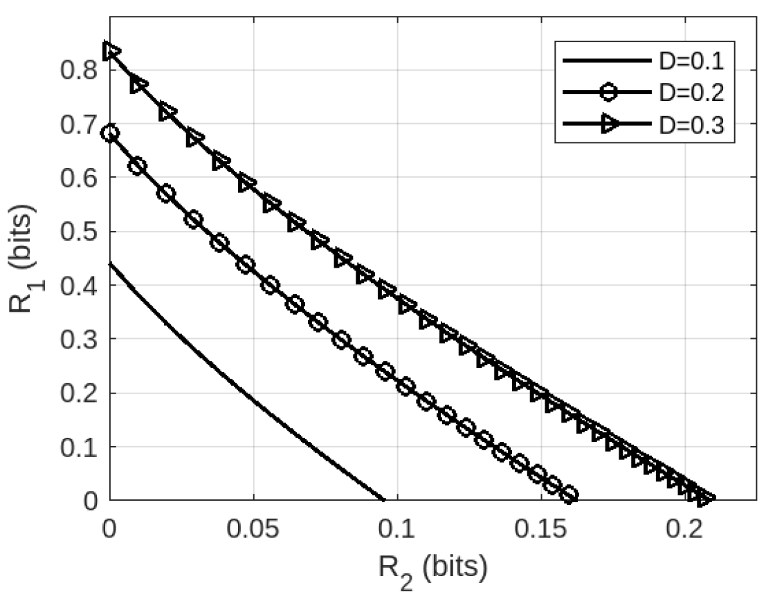
We now plot the trade=off region in Theorem 2 for an example system with the parameters [TeX:] $$p=0.4, q_1=2 / 9,$$ and [TeX:] $$q_2=4 / 9$$ in Fig. 2. In particular, we plot the tradeoff between the communication rates [TeX:] $$R_1 \text { and } R_2$$ for three fixed values of the input reconstruction distortion D. It is seen that demanding smaller distortion values (which amounts to a better quality input reconstruction) results in smaller achievable communication rates, and vice versa. For instance, the set of achievable rate pairs [TeX:] $$R_1 \text { and } R_2$$ for D = 0.1 (which corresponds to a better quality input reconstruction) are much smaller compared to the corresponding achievable rates for D = 0.3 (which corresponds to a poorer quality input reconstruction).

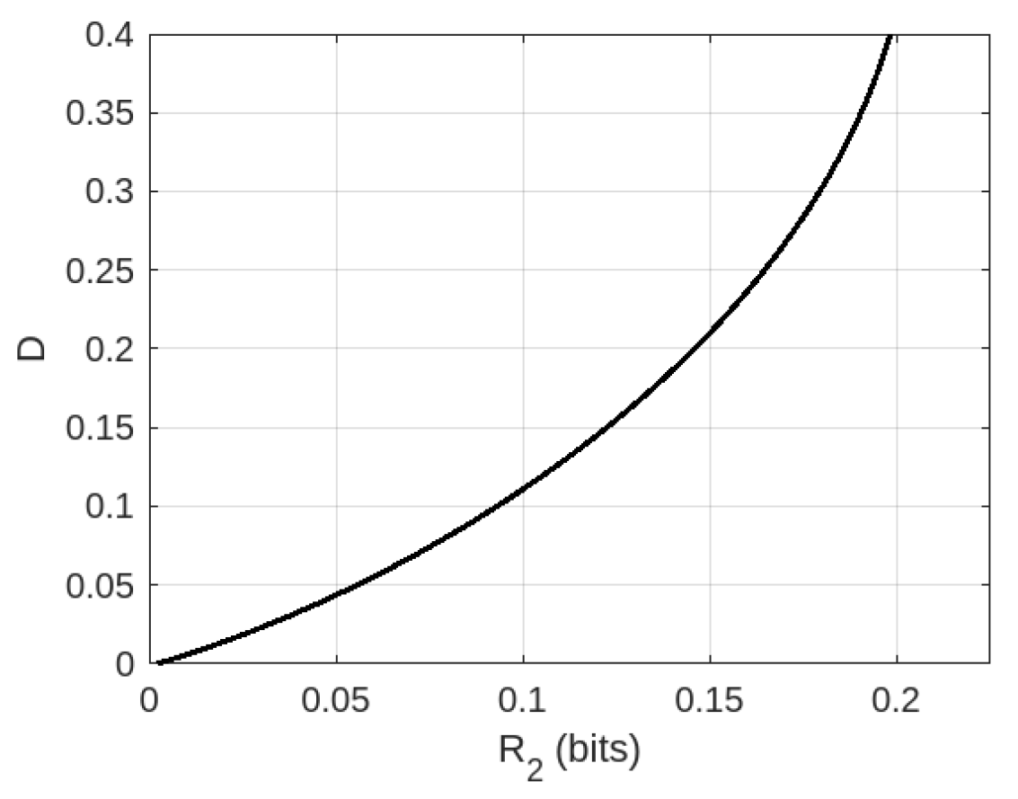
We have also plotted the trade-off between [TeX:] $$R_2$$ and D for the same parameters in Fig. 3, wherein it is observed that a higher D in fact leads to a higher [TeX:] $$R_2$$ (and vice-versa). This is unlike a traditional rate-distortion trade-off, where a higher description rate leads to a lower distortion. In contrast, the demand for a higher rate in our setting leads to a poorer quality input codeword estimate at the second receiver, i.e. a higher D (and vice-versa). This is because of the intrinsic tension between the dual requirements at the second receiver.

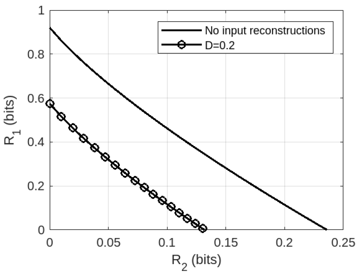
We also compare the region in Theorem 2 to the corresponding setting without any input reconstruction constraints, as depicted in Fig. 4. Naturally, it is observed that the introduction of an input reconstruction constraint restricts the region of achievable rates. In other words, larger rates are seen to be achievable in the absence of the input reconstruction constraint.

VI. CONCLUSION

A state-dependent degraded broadcast channel with input reconstruction requirements was investigated, and the optimal trade-off between the message communication rates and the input reconstruction distortion was characterized. The setting where the strong receiver is also uninformed of the state process appears to be an interesting and challenging problem for further investigations.

VII. ACKNOWLEDGEMENTS

The author would like to thank the Editor and two anonymous reviewers for their insightful comments, which has greatly helped the content and presentation of this paper.

APPENDIX A

PROOF OF CARDINALITY BOUND ON [TeX:] $$|\mathcal{U}|$$

In this section, we shall prove the cardinality bound on the auxiliary random variable U in Theorem 1, thereby showing that our characterization is computable. We use standard cardinality bounding techniques in the information theory literature, see [26]. We shall prove that [TeX:] $$|\mathcal{U}| \leq|\mathcal{S}| \cdot|\mathcal{X}|+2 . \text { Let } U \sim F(u)$$ and [TeX:] $$(S, X) \mid U=u \sim p(s, x \mid u),$$ where U takes values in [TeX:] $$\mathcal{U}$$. Given (U, S,X), consider the following [TeX:] $$|\mathcal{S}| \cdot|\mathcal{X}|+2$$ continuous real-valued functions of [TeX:] $$\pi=p(s, x \mid u)$$

By the Fenchel-Eggleston strengthening of Caratheodory’s theorem [26], there exists a random variable [TeX:] $$U^{\prime} \text { with }\left|\mathcal{U}^{\prime}\right| \leq |\mathcal{S}| \cdot|\mathcal{X}|+2$$ such that [TeX:] $$p(s, x), \mathbb{E}[d(X, \hat{X}) \mid U], H\left(Y_1 \mid U, S\right)$$ and [TeX:] $$H(S \mid U)-H\left(Y_2 \mid U\right)$$ are preserved:

We can thus write the following:

Moreover, it follows that:

Thus it suffices to consider auxiliary random variables U such that:

This completes the proof of the cardinality of the auxiliary random variable U in Theorem 1.

References

- 1 C. E. Shannon, "Channels with side information at the transmitter," IBM J. Research Development, vol. 2, no. 4, pp. 289-293, 1958.doi:[[[10.1147/rd.24.0289]]]
- 2 A. V . Kuznetsov and B. S. Tsybakov, "Coding in a memory with defective cells," Prob. peredachi informatsii, vol. 10, no. 2, pp. 52-60, 1974.custom:[[[-]]]
- 3 S. Gelfand and M. Pinsker, "Coding for channels with random parameters," Probl. Contr. Inform. Theory, vol. 9, no. 1, pp. 19-31, 1980.custom:[[[-]]]
- 4 C. Heegard and A. Gamal, "On the capacity of computer memory with defects," IEEE Trans. Inform. Theory, vol. 29, no. 5, pp. 731-739, 1983.doi:[[[10.1109/TIT.1983.1056723]]]
- 5 G. Caire and S. Shamai, "On the capacity of some channels with channel state information," IEEE Trans. Inform. Theory, vol. 45, no. 6, pp. 2007-2019, 1999.doi:[[[10.1109/18.782125]]]
- 6 Y . Steinberg, "Coding for the degraded broadcast channel with random parameters, with causal and noncausal side information," IEEE Trans. Inform. Theory, vol. 51, no. 8, pp. 2867-2877, 2005.doi:[[[10.1109/TIT.2005.851727]]]
- 7 G. Keshet, Y . Steinberg, and N. Merhav, "Channel coding in the presence of side information," Foundations Trends Commun. Inform. Theory, vol. 4, no. 6, pp. 445-586, 2007.doi:[[[10.1561/0100000025]]]
- 8 A. Sutivong, M. Chiang, T. M. Cover, and Y .-H. Kim, "Channel capacity and state estimation for state-dependent Gaussian channels," IEEE Trans. Inform. Theory, vol. 51, no. 4, pp. 1486-1495, 2005.doi:[[[10.1109/TIT.2005.844108]]]
- 9 M. H. Costa, "Writing on dirty paper (corresp.)," IEEE Trans. Inform. Theory, vol. 29, no. 3, pp. 439-441, 1983.doi:[[[10.1109/TIT.1983.1056659]]]
- 10 Y .-H. Kim, A. Sutivong, and T. M. Cover, "State amplification," IEEE Trans. Inform. Theory, vol. 54, no. 5, pp. 1850-1859, 2008.doi:[[[10.1109/TIT.2008.920242]]]
- 11 C. Choudhuri, Y .-H. Kim, and U. Mitra, "Causal state communication," IEEE Trans. Inform. Theory, vol. 59, no. 6, pp. 3709-3719, 2013.doi:[[[10.48550/arXiv.1203.6027]]]
- 12 V . Ramachandran, S. R. B. Pillai, and V . M. Prabhakaran, "Joint state estimation and communication over a state-dependent Gaussian multiple access channel," IEEE Trans. Commun., vol. 67, no. 10, pp. 6743-6752, 2019.doi:[[[10.1109/TCOMM.2019.2932069]]]
- 13 N. Merhav and S. Shamai, "Information rates subject to state masking," IEEE Trans. Inform. Theory, vol. 53, no. 6, pp. 2254-2261, 2007.doi:[[[10.1109/TIT.2007.896860]]]
- 14 O. O. Koyluoglu, R. Soundararajan, and S. Vishwanath, "State amplification subject to masking constraints," IEEE Trans. Inform. Theory, vol. 62, no. 11, pp. 6233-6250, 2016.doi:[[[10.48550/arXiv.1112.4090]]]
- 15 Y .-K. Chia, R. Soundararajan, and T. Weissman, "Estimation with a helper who knows the interference," IEEE Trans. Inform. Theory, vol. 59, no. 11, pp. 7097-7117, 2013.doi:[[[10.48550/arXiv.1203.4311]]]
- 16 C. Tian, B. Bandemer, and S. Shamai, "Gaussian state amplification with noisy observations," IEEE Trans. Inform. Theory, vol. 61, no. 9, pp. 4587-4597, 2015.doi:[[[10.1109/TIT.2015.2454519]]]
- 17 Y . Steinberg, "Coding and common reconstruction," IEEE Trans. Inform. Theory, vol. 55, no. 11, pp. 4995-5010, 2009.doi:[[[10.1109/TIT.2009.2030487]]]
- 18 K. Kittichokechai, T. J. Oechtering, and M. Skoglund, "Coding with action-dependent side information and additional reconstruction requirements," IEEE Trans. Inform. Theory, vol. 61, no. 11, pp. 6355-6367, 2015.doi:[[[10.48550/arXiv.1202.1484]]]
- 19 P. Grover, A. B. Wagner, and A. Sahai, "Information embedding and the triple role of control," IEEE Trans. Inform. Theory, vol. 61, no. 4, pp. 1539-1549, 2015.doi:[[[10.1109/TIT.2015.2402279]]]
- 20 C. Choudhuri and U. Mitra, "On Witsenhausen’s counterexample: The asymptotic vector case," in Proc. IEEE ITW, 2012.doi:[[[10.1109/ITW.2012.6404649]]]
- 21 O. Sumszyk and Y . Steinberg, "Information embedding with reversible stegotext," in Proc. IEEE ISIT, 2009.doi:[[[10.1109/ISIT.2009.5205855]]]
- 22 B. Bandemer and A. El Gamal, "Communication with disturbance constraints," IEEE Trans. Inform. Theory, vol. 60, no. 8, pp. 4488-4502, 2014.doi:[[[10.1109/ISIT.2011.6033924]]]
- 23 W. Zhang, S. Vedantam, and U. Mitra, "Joint transmission and state estimation: A constrained channel coding approach," IEEE Trans. Inform. Theory, vol. 57, no. 10, pp. 7084-7095, 2011.doi:[[[10.1109/TIT.2011.2158488]]]
- 24 P. Moulin and J. A. O’Sullivan, "Information-theoretic analysis of information hiding," IEEE Trans. Inform. Theory, vol. 49, no. 3, pp. 563-593, 2003.doi:[[[10.1109/TIT.2002.808134]]]
- 25 A. El Gamal and Y .-H. Kim, Network information theory. Cambridge University Press, 2011.custom:[[[-]]]
- 26 M. Salehi, "Cardinality bounds on auxiliary variables in multiple-user theory via the method of ahlswede and körner," Dept. Stat., Stanford Univ., Stanford, CA, Tech. Rep, vol. 33, 1978.custom:[[[-]]]