Daniel Kariuki Waweru , Fengfan Yang , Chunli Zhao , Lawrence Muthama Paul and Hongjun Xu
Distributed Totally Decomposed Cumulative Goppa Coded-Cooperative Communication with Optimized Selection in the Relay
Abstract: In this paper, powerful induced-cyclic totally decom- posed cumulative Goppa (TDCG) codes are selected and used for coded-cooperative diversity, which can fit wireless communication applications. Two TDCG codes employed at the source and relay nodes establish the joint design of the destination channel code. In the cooperation phase, we consider an optimized relay channel code which improves the overall bit-error-rate (BER) performance. Two methods of optimization are explored. The most practical method for optimization in terms of reduced processing complexity is proposed. We use a joint decoding which exploits all the resources gained by the cooperation scheme at the destination. The BER performance is evaluated through Monte-Carlo simulations with BPSK modulation and coherent detection over the flat Rayleigh fading channel. The proposed TDCG coded-cooperative diversity scheme exhibit a better BER performance than the non-cooperation scheme and other existing coded cooperation methods of similar code rates under similar channel conditions.
Keywords: Coded-cooperative communication system , joint decoding , optimized relay channel , totally decomposed cumulative Goppa codes
I. INTRODUCTION
MULTIPATH fading occurs due to multiple paths of radio signals from the transmitter to the receiver. The multipath fading is one of the substantial factors that degrade the performance of wireless communication systems. One method of mitigating multi-path fading is integrating the diversity technique, where the same signal appears in multiple instances in time, frequency, or antennas that fade independently. Node cooperation is an effective way of providing diversity in wireless networks [1], [2], whereby, exploiting the inherent broadcast nature of the wireless channel same information signal get distributed to two or more users who then cooperatively transmit it to a common destination. Node cooperation transmission scheme innately work as a virtual multiple input multiple output (MIMO) with distributed antennas (i.e., relays or cooperating users). In contrast to MIMO systems, however, the relay node is constrained to work in half-duplex mode, i.e., the node can either transmit or receive information signal at a time.
Recently, the integration of node cooperation with channel codes employed at the source and relay nodes has proven to be a beneficial technique to enhance the performance of the wireless system by improving the error-correction capability [3], [4]. Coded-cooperative communication is an enhanced decode-and-forward (DF) relaying technique [2], where two or more error control codes employed at the source and relay nodes jointly construct the destination code, which allows for joint decoding. Coded-cooperative communications bring higher data throughput, spectral and power efficiency, and reliability.
Many coded-cooperative diversity schemes already exit, such as Reed-Muller (RM) codes [5], Reed Solomon (RS) codes [6], low density parity check (LDPC) codes [4], [7], turbo codes [8], [9] and polar codes [10]–[12]. In this paper, we apply a ‘best-known’ linear algebraic code in codedcooperative communication. A linear code is said to be the “best-known linear code” if it has the highest minimum weight among all known linear codes of the same length and rate. The minimum Hamming distance and the weight spectrum are the two most important performance indicators of linear codes [13]. Given that a decoding algorithm, which can realize the full performance of a linear code exists, the best-known linear code offers better error rate performance. For a given code, the higher the minimum Hamming distance of the code, the better the performance. Moreover, in contrast to all past research and findings, another unique issue used in this study is an optimization method at the relay node based on the minimum Hamming distance and the weight spectrum of the jointly constructed destination code. We present an efficient algorithm for designing the optimized channel code at the relay. The optimized relaying accord improved cooperation in the coded-cooperative scheme. Hence, the paper is devoted to studying the coded-cooperative communication system, based on a subclass of classical Goppa codes, called the totally decomposed cumulative Goppa (TDCG) codes, in a three-node network comprising a source, a single relay and a destination.
Let [TeX:] $$q=p^m$$ with p a prime number and [TeX:] $$m \quad \in \quad \mathbb{N}^*, \quad G(x) \in \mathbb{F}_q[x]$$ be of degree s, and [TeX:] $$L=\left\{\gamma_i: 0 \leq i \leq n-1\right\} \subseteq \mathbb{F}_q$$, [TeX:] $$\gamma_i \neq \gamma_j$$ for [TeX:] $$i \neq j$$. Assume that L does not contain a root of [TeX:] $$G(x)$$, then a classical Goppa code, denoted as [TeX:] $$\Gamma(L, G(x))$$, is an [n, k, d] linear code defined as the set of all vectors [TeX:] $$\mathbf{c}=\left[c_0, c_1, \cdots, c_{n-1}\right]$$ with components in [TeX:] $$\mathbb{F}_p$$ which satisfy the condition
The set L is called the locator set and its cardinality defines the length n of [TeX:] $$\Gamma(L, G(x))$$. The polynomial [TeX:] $$G(x)$$ is called the Goppa polynomial. The dimension of [TeX:] $$\Gamma(L, G(x))$$ is [TeX:] $$k \geq n-m s$$ and the minimal Hamming distance d satisfies [TeX:] $$d \geq s+1$$, called the Goppa bound. The classical Goppa code, whose codewords have components in [TeX:] $$\mathbb{F}_p,$$ is a subfield subcode of a generalized Reed-Solomon (GRS) code defined in an extension field [TeX:] $$\mathbb{F}_p$$ of [TeX:] $$\mathbb{F}_p$$ [14]. They were first introduced in 1970 by Goppa [15], and are well known to be non-cyclic in general [16]. Goppa construction is more powerful as we are sure that there are families of Goppa codes that reach the Gilbert-Varshamov bound [17], [18] and that many binary Goppa codes are placed in the table of the best-known linear codes [19]. The Goppa codes are easy to encode and decode [17], [20] and hence are quite practical for implementation. Goppa [15] also introduces four important subclasses of Goppa codes based on the form of a Goppa polynomial: [TeX:] $$\Gamma(L, G(x))$$ is a cyclic code when [TeX:] $$G(x)=x^s$$, a separable code when [TeX:] $$G(x)$$ is a separable polynomial, an irreducible code when [TeX:] $$G(x)$$ is an irreducible polynomial, and a cumulative Goppa code when [TeX:] $$G(x)=(x-\beta)^s$$. In 1976, Sugiyama et al. [21] considered some generalization of cumulative binary Goppa codes with Goppa polynomials: [TeX:] $$G_1(x)=g(x)^q$$ and [TeX:] $$G_2(x)=g(x)^{(q-1)}$$, where [TeX:] $$g(x)$$ is a separable polynomial. A Goppa code [TeX:] $$\Gamma(L, G(x))$$ with [TeX:] $$G(x)=(x-\beta)^s$$ and [TeX:] $$L \subseteq \mathbb{F}_q \backslash\{\beta: G(\beta)=0\}$$, where [TeX:] $$G(x)$$ is a polynomial totally decomposed in [TeX:] $$\mathbb{F}_p$$, is called a TDCG code [22]. The parameter s is called the order of cumulativity of this code. The corresponding TDCG code will be denoted as [TeX:] $$\Gamma(L, G(x), s)$$. It turns out that the TDCG code [TeX:] $$\Gamma(L, G(x), s)$$ can be made to define a cyclic code by appropriately selecting the locator set L [23]–[25]. The cyclic property of the [TeX:] $$\Gamma(L, G(x), s)$$-code is induced by some semilinear transformation [TeX:] $$f \in P \Gamma L\left(2, \mathbb{F}_q\right)$$ of the underlying GRS code. The action of f over [TeX:] $$L=\left\{\gamma_0, \gamma_1, \cdots, \gamma_{n-1}\right\}$$ is defined as
(1)
[TeX:] $$L^f=\left\{f\left(\gamma_0\right), f\left(\gamma_1\right), \cdots, f\left(\gamma_{n-1}\right)\right\},$$where [TeX:] $$\gamma_{\sigma(i)}=f\left(\gamma_i\right)$$ and a permutation of a permutation of [TeX:] $$\{0,1, \cdots, n-1\}$$ [26], [23]. The parameters of the cyclic TDCG codes we use in this research are such as those of the best-known linear cyclic codes [22], [19].
This paper utilizes the cyclic TDCG codes in a coded-cooperative diversity scheme. TDCG coded-cooperative schemes are suitable for use in a wide range of upcoming short- and medium-range (i.e., a few centimetres to several hundreds of meters) wireless devices. These devices, the majority of which are Internet of things (IoT) and mobile internet, are now a part of our daily lives and connect people to one another and their environments. Our suggested codedcooperative scheme based on TDCG codes can be applied to critical short- and medium-range IoT applications that relate to the low-cost, massive in number, and low-powered devices communication among themselves [27]. Such IoT characterizes a wide range of technologies, such as smart metering, advanced wearables, logistics and body sensors, massive automated cities and industrial control and monitoring. The codedcooperative networks, which can encompass these massiveaccess networks, require high-efficient short/medium block length channel codes (i.e., codes with information words of length 50 to 1000 bits). The TDGC code is a superior candidate for these coded-cooperative massive-access wireless networks.
A totally decomposed cumulative Goppa codedcooperative (TDCGCC) diversity scheme for a single relay scenario has two cyclic TDCG codes placed at the source and relay cooperatively communicating with a common destination and operate in a two-time-slot transmission. The time-division-based half-duplex relaying is chosen because of its practical utility. The importance of the resources made available by relay optimization is shown through joint decoding using naive and smart algorithms. It is also assumed that in the coded-cooperation scenario, the transmissions from source-to-destination (S-D), from source-to-relay (S-R) and relay-to-destination (R-D) links do not employ orthogonal channels. The use of the nonorthogonal channel models is motivated by the fact that it offers a higher channel capacity than the cooperation schemes assuming orthogonal channels [28]. Monte-Carlo simulations show that the proposed TDCGCC scheme significantly outperforms the non-cooperation scheme and other existing coded cooperation methods of similar code rates under similar channel conditions. The general assumptions made for simulations are: all corresponding receivers have perfect channel side information, BPSK modulation is used at all the transmit nodes, and each transmission scheme transmits at an equal power for a fair comparison. One key issue used in this paper is the match between our binary error-correction codes and the BPSK modulation scheme. However, appropriate higher modulation schemes can be inferred for specific short and medium-range wireless communication application requirements.
The remainder of this manuscript is structured as follows. The overall description of a single relaying coded-cooperative method is provided in Section II. The TDCG codes and system model for a single relay TDCGCC scheme are described in Section III. The optimization process and effective algorithm utilized to create an optimized relay channel code are described in Section IV. The joint decoding based on naive and smart algorithms is described in Section V. The results of the numerical simulation are provided in Section VI. The paper is concluded in Section VII. This manuscript’s main contributions are:
1) Investigate the feasibility of using TDCG codes in cooperative systems.
2) Implement an optimization criterion in the relay node and evaluate the performance of the suggested cooperative scheme against the non-cooperative scheme.
3) Evaluate the performance of the proposed codedcooperative in a practical scenario.
4) Evaluate the performance of TDCG codes in comparison to Bose–Chaudhuri–Hocquenghem (BCH) codes and other existing coded cooperation methods of similar rates under similar channel conditions.
II. GENERAL DESCRIPTION OF SINGLE RELAY CHANNEL CODING SCHEME
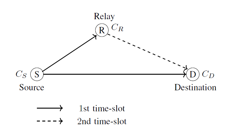
An elementary three-node network [29] with a source, a single relay, and a destination is depicted in Fig. 1. The relay has been positioned intentionally closer to the source than the destination is to the source. We now describe our coding strategy operating in a two-time-slot transmission. Two linear codes are used at the source and relay, as was previously mentioned. The first code [TeX:] $$C_S\left(n_1, k_1, d_1\right)$$ with a generator matrix [TeX:] $$\mathrm{G}_S$$ is employed by the source. A code-word [TeX:] $$\mathbf{c}_1=\left[c_0, c_1, \cdots, c_{n_1-1}\right]$$ is generated from the message block [TeX:] $$\mathbf{m}_1=\left[m_0, m_1, \cdots, m_{k_1-1}\right]$$, i.e., [TeX:] $$\mathbf{c}_1=\mathbf{m}_1 \mathbf{G}_S$$, where [TeX:] $$m_l, c_s \in \mathbb{F}_q, 0 \leq l \leq k_1-1,0 \leq s \leq n_1-1,$$ and [TeX:] $$q=p^k$$ with p a prime number and [TeX:] $$k \in \mathbb{N}^* \text {. }$$ In the 1st time slot, the source transmits all [TeX:] $$n_1$$ coded information bits to the relay and destination over noisy channels simultaneously. This phase is called broadcast transmission. The second code [TeX:] $$C_R\left(n_2, k_2, d_2\right) \quad\left(k_2 \leq k_1\right)$$ with the generator matrix [TeX:] $$\mathbf{G}_R$$ is employed by the relay. In the 2nd time slot, the relay decodes the noise-corrupted observation [TeX:] $$\hat{\mathbf{r}}_1$$ to obtain a codeword [TeX:] $$\hat{\mathbf{c}}_1 \in C_S$$ and then obtains the estimated message block [TeX:] $$\hat{\mathbf{m}}_1=\left[\hat{m}_0, \hat{m}_1, \cdots, \hat{m}_{k_1-1}\right], \hat{m}_l \in \mathbb{F}_q .$$ Assuming that the relay channel code has already been optimized (see Section IV), the relay selects [TeX:] $$k_2$$ out of [TeX:] $$k_1$$ decoded bits of [TeX:] $$\hat{\mathbf{m}}_1$$ as its own message [TeX:] $$\mathbf{m}_2$$, based on the optimal selection pattern, and instantaneously re-encodes it into [TeX:] $$\mathbf{c}_2=\mathbf{m}_2 \mathbf{G}_R$$. Then, [TeX:] $$\mathbf{C}_2$$ is sent to the destination over the noisy channel. This second phase is called cooperation transmission. The destination gathers the [TeX:] $$n_1+n_2$$ noise-corrupted observations received in the two phases as a single block [TeX:] $$\left[\hat{\mathbf{r}}_1, \hat{\mathbf{r}}_2\right]$$ and decodes it. So, the following is the destination code:
(2)
[TeX:] $$\begin{aligned} C_D\left(n_1+n_2, k_1\right)= & \left\{\left[\mathbf{c}_1, \mathbf{c}_2\right] \mid \mathbf{c}_1=\mathbf{m}_1 \mathbf{G}_S\right., \\ & \mathbf{c}_2=\mathbf{m}_2 \mathbf{G}_R, \mathbf{m}_1 \in \mathbb{F}_q^{k_1}, \\ & \left.\mathbf{m}_2 \in \mathbb{F}_q^{k_2}\right\}. \end{aligned}$$The observation [TeX:] $$\left[\hat{\mathbf{r}}_1, \hat{\mathbf{r}}_2\right]$$ is decoded into some codeword [TeX:] $$\left[\hat{\mathbf{c}}_1, \hat{\mathbf{c}}_2\right] \in C_D$$ by joint decoding. The code rate of [TeX:] $$C_D$$ is [TeX:] $$k_1 / n_1+n_2$$, and its minimum Hamming distance, called the free distance, denoted as [TeX:] $$d_{\text {free }}$$, is highly dependent on the message symbol selection at the relay. More details are given in Section IV.
III. SINGLE RELAY TDCG CODING SCHEME WITH A SUBCODE DESIGN AT THE DESTINATION
A. TDCG Codes with Very Good Parameters
In Section I, induced-cyclic TDCG codes were introduced. In this paper, we will only be concerned with induced-cyclic TDCG codes [TeX:] $$\Gamma(L, G(x), s)$$ of length [TeX:] $$n=q^2+q+1$$ which are explicitly defined as follows. Consider a finite Galois cubic field [TeX:] $$\mathbb{F}_{q^3}$$, with [TeX:] $$q=p^m$$. The Goppa code [TeX:] $$\Gamma(L, G(x), s)$$ of length [TeX:] $$n=q^2+q+1$$ has a Goppa polynomial of the form [TeX:] $$G(x)=(x+\beta)^s$$ with [TeX:] $$\beta=\gamma^n$$, for some primitive element [TeX:] $$\gamma \in \mathbb{F}_{q^3}$$. The locator set [TeX:] $$L \subset \mathbb{F}_{q^3}$$ is a single n-cycle set generated by [TeX:] $$f \in P \Gamma L\left(2, \mathbb{F}_q\right)$$ such that [TeX:] $$L=\left\{\gamma_0, \gamma_1, \cdots, \gamma_{n-1}\right\}$$, [TeX:] $$\gamma_i \neq \gamma_j$$ for [TeX:] $$i \neq j, \gamma_{n-1}=1, \gamma_i^n=\gamma_i^{-1}=\gamma_{n-2-i}$$ for all [TeX:] $$0 \leq i \leq n-2$$, and
(3)
[TeX:] $$\gamma_{(i \bmod n)+1}=f\left(\gamma_i\right)=\frac{\gamma_i\left(\frac{1+\beta^2 \mu}{\beta-\beta \mu}\right)+1}{\gamma_i+\left(\frac{\mu+\beta^2}{\beta-\beta \mu}\right)}$$where is an nth root of unity and is [TeX:] $$\left(\left(q^3-1\right) / n\right)$$th root of unity. The [TeX:] $$\Gamma(L, G(x), s)$$-codes have excellent estimations of the minimum distance and dimension, as well as parameters that are such as those of the best-known codes [19].
To demonstrate our proposed coding scheme, we first consider short cyclic TDCG codes of length n = 21 over [TeX:] $$\mathbb{F}_{2^{12}}$$ with the elements of its locator set L having the ordering: [TeX:] $$\gamma_{i+1}=\frac{\gamma_i \cdot \gamma^{1731}+1}{\gamma_i+\gamma^{1265}}$$ for [TeX:] $$i=1, \cdots, 20 \text {, and } \gamma_{21}=1 \text {, }$$ i.e.,
Secondly, we use relatively longer cyclic TDCG codes of length n = 73 over [TeX:] $$\mathbb{F}_{2^9}$$ with the elements of the locator set L having the ordering: [TeX:] $$\gamma_{i+1}=\frac{\gamma_i \cdot \gamma^{126}+1}{\gamma_i+\gamma^{200}}$$ for [TeX:] $$i=1, \cdots, 72 \text {, and } \gamma_{73}=1 \text {, }$$ i.e.,
Table I give the TDCG codes exploited in the various TDCGCC schemes presented in Table II. The same n-cycle locator set has been used to define all TDCG codes of the same length.
TABLE I
| [TeX:] $$G(x)$$ | [TeX:] $$\Gamma(L, G(x), s)$$ | The weight spectrum of [TeX:] $$\Gamma(L, G(x), s)$$ |
|---|---|---|
| [TeX:] $$(x+\beta)^1$$ | [TeX:] $$[21,14,4]_2$$ | [1, 0, 0, 0, 84, 0, 924, 0, 2982, 0, 5796, 0, 4340, 0, 1956, 0, 273, 0, 28, 0, 0, 0]. |
| [TeX:] $$(x+\beta)^3$$ | [TeX:] $$[21,11,6]_2$$ | [1, 0, 0, 0, 0, 0, 168, 0, 210, 0, 1008, 0, 280, 0, 360, 0, 21, 0, 0, 0, 0, 0]. |
| [TeX:] $$(x+\beta)^5$$ | [TeX:] $$[21,5,10]_2$$ | [1, 0, 0, 0, 0, 0, 0, 0, 0, 0, 21, 0, 7, 0, 3, 0, 0, 0, 0, 0, 0, 0]. |
| [TeX:] $$(x+\beta)^7$$ | [TeX:] $$[21,3,12]_2$$ | [1, 0, 0, 0, 0, 0, 0, 0, 0, 0, 0, 0, 7, 0, 0, 0, 0, 0, 0, 0, 0, 0]. |
| [TeX:] $$(x+\beta)^11$$ | [TeX:] $$[73,27,20]_2$$ | [1, 0, 0, 0, 0, 0, 0, 0, 0, 0, 0, 0, 0, 0, 0, 0, 0, 0, 0, 0, 26280, 0, 0, 0, 667293, 0, 0, 0, 6981136,0, 0, 0, 28840329, 0, 0, 0, 49665696, 0, 0, 0, 35826210, 0, 0, 0, 10837872, 0, 0, 0,1307430, 0, 0, 0, 64824, 0, 0, 0, 657, 0, 0, 0, 0, 0, 0, 0, 0, 0, 0, 0, 0, 0, 0, 0, 0, 0]. |
| [TeX:] $$(x+\beta)^13$$ | [TeX:] $$[73,18,24]_2$$ | [1, 0, 0, 0, 0, 0, 0, 0, 0, 0, 0, 0, 0, 0, 0, 0, 0, 0, 0, 0, 0, 0, 0, 0, 1533, 0, 0, 0, 12629, 0, 0, 0, 59130, 0, 0, 0, 92929, 0, 0, 0, 72927, 0, 0, 0, 20367, 0, 0, 0, 2409, 0, 0, 0, 219, 0, 0, 0, 0, 0, 0, 0, 0, 0, 0, 0, 0, 0, 0, 0, 0, 0, 0, 0, 0, 0]. |
TABLE II
| Serial | [TeX:] $$C_S$$ | [TeX:] $$C_R$$ | [TeX:] $$C_D$$ | [TeX:] $$d_{\text {free }}$$ | Rate (R) |
|---|---|---|---|---|---|
| [TeX:] $$M_1$$ | [21, 5, 10] | [21, 3, 12] | [42, 5] | 10 | 0.1190 |
| [TeX:] $$M_2$$ | [21, 14, 4] | [21, 11, 6] | [42, 14] | 4 | 0.3333 |
| [TeX:] $$M_3$$ | [73, 27, 20] | [73, 18, 24] | [146, 27] | 20 | 0.1849 |
B. System Model
1) Cooperative scheme: Fig. 2 illustrates the single relay TDCG coding scheme. Two cyclic TDCG codes are used in the TDCG coding system, [TeX:] $$C_S$$ at the source and [TeX:] $$C_R$$ at the relay, and they both operate over a Rayleigh fading channel.
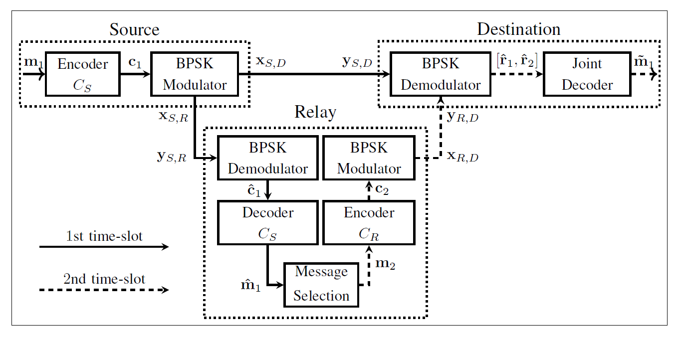
The message sequence [TeX:] $$\mathrm{m}_1$$ is encoded to the codeword [TeX:] $$\mathbf{c}_1 \in C_S$$ during the 1st time slot, and the source simultaneously broadcasts the coded modulated symbol sequences [TeX:] $$\mathbf{x}_{S, R}=\left[x_{S, R}^0, x_{S, R}^1, \cdots, x_{S, R}^{n_1-1}\right]$$ to the relay node and [TeX:] $$\mathbf{x}_{S, D}=\left[x_{S, D}^0, x_{S, D}^1, \cdots, x_{S, D}^{n_1-1}\right]$$ to the destination node. For each [TeX:] $$i=0,1, \cdots, n_1-1,$$ during the 1st time slot of the ith instant, i.e., [TeX:] $$i_1$$th time instant, the modulated symbols [TeX:] $$x_{S, R}^i$$ and [TeX:] $$x_{S, D}^i$$ are transmitted to their respective nodes over the Rayleigh fading channel. The received signals [TeX:] $$y_{S, R}^i$$ at the relay node and [TeX:] $$y_{S, D}^i$$ at the destination node are given by:
The [TeX:] $$h_{S, R}^i$$ (respectively, [TeX:] $$h_{S, D}^i$$) represents the channel coefficient owing to Rayleigh fading, a complex Gaussian variable with a zero mean and 0.5 variance per dimension. The [TeX:] $$n_{S, R}^i$$ (respectively, [TeX:] $$n_{S, D}^i$$) represents the additive white Gaussian noise, a complex Gaussian variable with a zero mean and 0.5 variance per dimension. After transmitting all the [TeX:] $$n_1$$ modulated symbols, the received signal sequences: At the relay node is denote by [TeX:] $$\mathbf{y}_{S, R}=\left[y_{S, R}^0, y_{S, R}^1, \cdots, y_{S, R}^{n_1-1}\right],$$ and at the destination node is denoted [TeX:] $$\mathbf{y}_{S, D}=\left[y_{S, D}^0, y_{S, D}^1, \cdots, y_{S, D}^{n_1-1}\right]$$.
During the 2nd time slot, the relay receives the estimated message [TeX:] $$\hat{\mathbf{m}}_1$$ from the source. The relay then selects the message sequence [TeX:] $$\mathbf{m}_2 \text { from } \hat{\mathbf{m}}_1$$, encodes it to the codeword [TeX:] $$\mathbf{c}_2 \in C_R$$ and broadcasts the coded modulated symbol sequence [TeX:] $$\mathbf{x}_{R, D}=\left[x_{R, D}^0, x_{R, D}^1, \cdots, x_{R, D}^{n_2-1}\right]$$ to the destination node. The received signal at the destination node during the [TeX:] $$i_2$$th time instant, for each [TeX:] $$i=0,1, \cdots, n_2-1$$, has the following form:
Here, [TeX:] $$h_{S, D}^i$$ and [TeX:] $$n_{R, D}^i$$ are defined similar to [TeX:] $$h_{S, R}^i$$ and [TeX:] $$n_{S, R}^i$$, respectively. After transmitting all the [TeX:] $$n_2$$ modulated symbols, the received signal sequence at the destination node is [TeX:] $$\mathbf{y}_{R, D}=\left[y_{R, D}^0, y_{R, D}^1, \cdots, y_{R, D}^{n_2-1}\right].$$
The overall received signal sequence at the destination node following the transmission of all the [TeX:] $$n_1+n_2$$ modulated symbols is given by [TeX:] $$\mathbf{y}=\left[\mathbf{y}_{S, D}, \mathbf{y}_{R, D}\right] .$$ Demodulating the signal [TeX:] $$\mathbf{y}$$ yields [TeX:] $$\hat{\mathbf{r}}=\left[\hat{\mathbf{r}}_1, \hat{\mathbf{r}}_2\right]$$, which is the initial likelihood of some codeword [TeX:] $$\left[\hat{\mathbf{c}}_1, \hat{\mathbf{c}}_2\right] \in C_D$$, with [TeX:] $$\hat{\mathbf{c}}_1 \in C_S$$ and [TeX:] $$\hat{\mathbf{c}}_2 \in C_R$$. If the relay selects its [TeX:] $$k_2$$ message sequence [TeX:] $$\mathbf{m}_2$$ independent of [TeX:] $$\hat{\mathbf{m}}_1$$ to generate the initial likelihood [TeX:] $$\hat{\mathbf{r}}_2^*$$, then through the joint construction, the destination obtains the initial likelihood [TeX:] $$\left[\hat{\mathbf{r}}_1, \hat{\mathbf{r}}_2^*\right]$$ of some codeword [TeX:] $$\left[\hat{\mathbf{c}}_1, \hat{\mathbf{c}}_2^*\right] \in \bar{C}_D$$. In this case, the optimized jointly-constructed destination code [TeX:] $$C_D$$ is a subcode of [TeX:] $$\bar{C}_D$$.
2) Non-cooperative scheme: Without a relay’s assistance, the source is transmitting the [TeX:] $$n_1$$ symbols in 5 to the destination. The received signal [TeX:] $$\mathbf{y}_{S, D}$$ is then demodulated into [TeX:] $$\hat{\mathbf{r}}_1$$, which represents the initial likelihood of some codeword [TeX:] $$\hat{\mathbf{c}}_1 \in C_S.$$
IV. OPTIMIZING SELECTION IN THE RELAY
In this section, we describe an optimization design criterion and an efficient algorithm to achieve the design objective. In order to explicitly state the related positions of each of the [TeX:] $$k_2$$ bits chosen from [TeX:] $$k_1$$ information bits, we will refer to the patterns produced by the combination [TeX:] $$\left(\begin{array}{l} k_1 \\ k_2 \end{array}\right)$$ as having an index
(7)
[TeX:] $$j \in \Lambda=\left\{1, \cdots,\left(\begin{array}{l} k_1 \\ k_2 \end{array}\right)\right\},$$where each j is in one-to-one correspondence to a distinct pattern, a [TeX:] $$k_2$$-tuple [TeX:] $$\boldsymbol{\Omega}_j=\left[l_1^{(j)}, \cdots, l_{k_2}^{(j)}\right],$$ that we will refer to as the jth selection pattern, where [TeX:] $$0 \leq l_1^{(j)}<\cdots<l_{k_2}^{(j)} \leq k_1-1$$. Thus, a set [TeX:] $$\Phi=\left\{\boldsymbol{\Omega}_j \mid j \in \Lambda\right\}$$ is formed by all of the selection patterns. The [TeX:] $$k_2$$ bits chosen from the [TeX:] $$k_1$$ decoded bits that correspond to each jth selection pattern [TeX:] $$\Omega_j$$ are denoted by the symbol [TeX:] $$\mathbf{m}_2^{(j)}=\left[m_0^{(j)}, m_1^{(j)}, \cdots, m_{k_2-1}^{(j)}\right],$$ with [TeX:] $$m_l^{(j)} \in \mathbb{F}_p$$. The jth selection pattern produces a destination code
(8)
[TeX:] $$\begin{aligned} & C_D^{(j)}\left(n_1+n_2, k_1\right)= \\ & \left\{\left[\mathbf{c}_1, \mathbf{c}_2^{(j)}\right] \mid \mathbf{c}_1=\mathbf{m}_1 \mathbf{G}_S, \mathbf{c}_2^{(j)}=\mathbf{m}_2^{(j)} \mathbf{G}_R\right\}, \end{aligned}$$whose minimum Hamming distance, which we call the free distance, is denoted as [TeX:] $$d_{\text {free}}^{(j)}.$$ For obtaining the optimal message bit selection pattern at the relay, the following optimization techniques are suggested.
A. Exhaustive Search
Consider the TDCGCC scheme [TeX:] $$M_1$$ defined in Table II. We have [TeX:] $$k_1=5, k_2=3, \Lambda=\left(\begin{array}{l} 5 \\ 3 \end{array}\right)=10$$, and the set of information selection patterns is
Table III is a list of the destination codes [TeX:] $$C_D^{(j)}$$ corresponding to various jth selection patterns. For each [TeX:] $$j \in \Lambda$$, we determine that the maximum free distance [TeX:] $$d_{\text {free }}^{(j)}=10$$. We should also point out that, even though the minimum Hamming distance of the code [TeX:] $$C_D^{(j)}(42,5)$$ is not improved, the weight spectrum get optimized in the sense that codewords of low weight in [TeX:] $$C_D^{(j)}(42,5)$$ are greatly reduced for every j as compared to the codewords of [TeX:] $$C_S(21,5,10)$$.
Let [TeX:] $$d_{\text {free }}^{(\operatorname{Max})}$$ be defined as follows:
(9)
[TeX:] $$d_{\text {free }}^{(\mathrm{Max})}=\max _j\left\{d_{\text {free }}^{(j)} \mid j \in \Lambda\right\} .$$At the relay, we seek the unique optimal bit selection pattern that allows the destination code [TeX:] $$C_D^{(j)}\left(n_1+n_2, k_1\right)$$ to achieve the maximum free distance [TeX:] $$d_{\text {free }}^{(j)}=d_{\text {free }}^{(\operatorname{Max})}$$. Thus, the resulting code and its free distance are thus denoted as [TeX:] $$C_D\left(n_1+n_2, k_1, d_{\text {free}}\right)$$, by dropping the index j, and the search is complete. From Table III, an optimum code, [TeX:] $$C_D(42,5)$$, in terms of highest free distance, can not be determined uniquely because all the destination codes [TeX:] $$C_D^{(j)}(42,5)$$, for each [TeX:] $$j \in \Lambda,$$ achieve the maximum free distance [TeX:] $$d_{\text {free }}^{(Max)}=10$$. A few more steps are required. Starting with [TeX:] $$i=0, d_{\text {free }}^{(j)}=d_{\text {free }}^{(j)}+0,$$ and such that [TeX:] $$d_1 \leq d_{\text {free }}^{(j)}+i \leq n_1 \text {, let } N_{d_{\text {free }}^{(j)}+i}$$ be the number of codewords of Hamming weight [TeX:] $$d_{\text {free }}^{(j)}+i \text { in } C_D^{(j)}\left(n_1+n_2, k_1\right).$$ The unique optimum code [TeX:] $$C_D\left(n_1+n_2, k_1, d_{\text {free }}\right)$$ is obtained by maximizing the [TeX:] $$d_{\text {free }}^{(j)}+i$$ while minimizing the [TeX:] $$N_{d_{\text {free }}^{(j)}+i}$$ among all candidates [TeX:] $$C_D^{(j)}\left(n_1+n_2, k_1\right), j \in \Lambda .$$ In Table IV, we obtain all the destination codes [TeX:] $$C_D^{(j)}(14,5)$$ associated with various selection patterns in for which [TeX:] $$d_{\text {free }}^{(j)}+0=10$$ and [TeX:] $$N_{d_{\text {free }}^{(j)}+0}=2.$$ Because both codes in Table IV have the same Hamming weight spectrum, either of them is optimal and will produce a fully optimized relay channel code.
TABLE III
| j | [TeX:] $$\Omega_j$$ | [TeX:] $$C_D^{(j)}(42,5)$$ | [TeX:] $$d_{\text {free }}^{(j)}$$ | The weight enumerator: [TeX:] $$w t_{(j)}(x)$$ |
|---|---|---|---|---|
| 1 | [TeX:] $$\Omega_1$$ | [TeX:] $$C_D^{(1)}(42,5)$$ | 10 | [TeX:] $$1+3 x^{10}+0 x^{12}+18 x^{22}+7 x^{24}+3 x^{26}$$ |
| 2 | [TeX:] $$\Omega_2$$ | [TeX:] $$C_D^{(2)}(42,5)$$ | 10 | [TeX:] $$1+2 x^{10}+1 x^{12}+19 x^{22}+6 x^{24}+3 x^{26}$$ |
| 3 | [TeX:] $$\Omega_3$$ | [TeX:] $$C_D^{(3)}(42,5)$$ | 10 | [TeX:] $$1+3 x^{10}+0 x^{12}+18 x^{22}+7 x^{24}+3 x^{26}$$ |
| 4 | [TeX:] $$\Omega_4$$ | [TeX:] $$C_D^{(4)}(42,5)$$ | 10 | [TeX:] $$1+3 x^{10}+0 x^{12}+18 x^{22}+7 x^{24}+3 x^{26}$$ |
| 5 | [TeX:] $$\Omega_5$$ | [TeX:] $$C_D^{(5)}(42,5)$$ | 10 | [TeX:] $$1+3 x^{10}+0 x^{12}+18 x^{22}+7 x^{24}+3 x^{26}$$ |
| 6 | [TeX:] $$\Omega_6$$ | [TeX:] $$C_D^{(6)}(42,5)$$ | 10 | [TeX:] $$1+3 x^{10}+0 x^{12}+18 x^{22}+7 x^{24}+3 x^{26}$$ |
| 7 | [TeX:] $$\Omega_7$$ | [TeX:] $$C_D^{(7)}(42,5)$$ | 10 | [TeX:] $$1+3 x^{10}+0 x^{12}+18 x^{22}+7 x^{24}+3 x^{26}$$ |
| 8 | [TeX:] $$\Omega_8$$ | [TeX:] $$C_D^{(8)}(42,5)$$ | 10 | [TeX:] $$1+2 x^{10}+1 x^{12}+19 x^{22}+6 x^{24}+3 x^{26}$$ |
| 9 | [TeX:] $$\Omega_9$$ | [TeX:] $$C_D^{(9)}(42,5)$$ | 10 | [TeX:] $$1+3 x^{10}+0 x^{12}+18 x^{22}+7 x^{24}+3 x^{26}$$ |
| 10 | [TeX:] $$\Omega_10$$ | [TeX:] $$C_D^{(10)}(42,5)$$ | 10 | [TeX:] $$1+3 x^{10}+0 x^{12}+18 x^{22}+7 x^{24}+3 x^{26}$$ |
TABLE IV
| j | [TeX:] $$\Omega_j$$ | [TeX:] $$C_D^{(j)}(42,5)$$ | [TeX:] $$d_{\text {free }}^{(j)}$$ | The weight enumerator: [TeX:] $$w t_{(j)}(x)$$ |
|---|---|---|---|---|
| 2 | [TeX:] $$\Omega_2$$ | [TeX:] $$C_D^{(2)}(42,5)$$ | 10 | [TeX:] $$1+2 x^{10}+1 x^{12}+19 x^{22}+6 x^{24}+3 x^{26}$$ |
| 8 | [TeX:] $$\Omega_8$$ | [TeX:] $$C_D^{(8)}(42,5)$$ | 10 | [TeX:] $$1+2 x^{10}+1 x^{12}+19 x^{22}+6 x^{24}+3 x^{26}$$ |
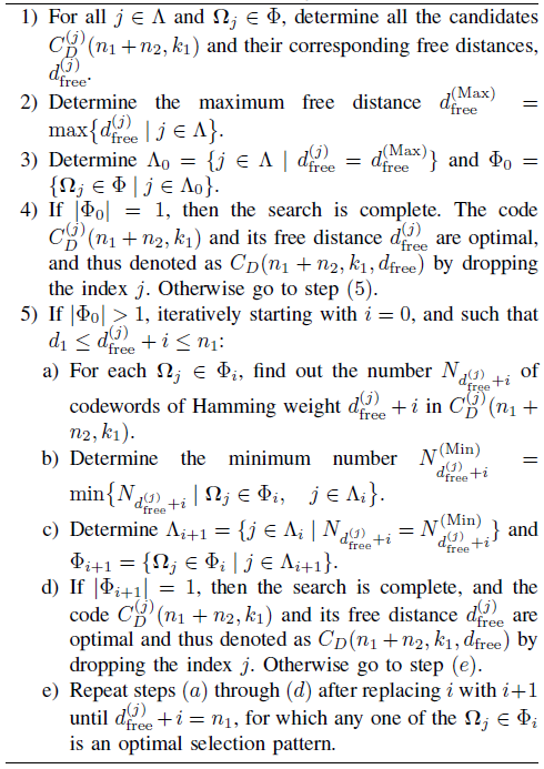
In general, the exhaustive search method comprises the precise steps enumerated in Algorithm 1. Although an exhaustive search guarantees an optimally designed relay channel code, the efficiency of this method decreases as the value of [TeX:] $$k_1$$ increases because the processing complexity of Algorithm 1 also increases. It is more practical to conduct a partial search for promising candidates. We will now go over the partial search method in detail.
B. Partial Search
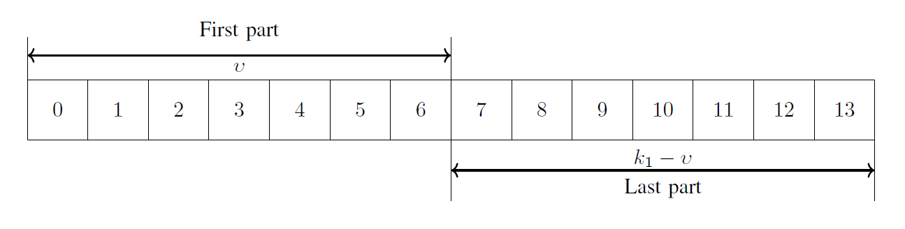
We suggest a division strategy that splits the [TeX:] $$k_1$$ decoded message bits at the relay into two nearly equal parts and two scenarios. This is illustrated in Fig. 3 for the TDCGCC scheme [TeX:] $$M_2$$. Define [TeX:] $$v=\left\lceil k_1 / 2\right\rceil=7$$ and let be an integer such that [TeX:] $$k_2 / 2<\mu \leq \min \left(v, k_2\right)$$. As a result, [TeX:] $$\mu \in\{6,7\}$$. In the division strategy, instead of selecting all [TeX:] $$k_2=11$$ bits from the [TeX:] $$k_1=14$$ bits available, which can be done in [TeX:] $$\left(\begin{array}{l} k_1 \\ k_2 \end{array}\right)=\left(\begin{array}{l} 14 \\ 11 \end{array}\right)=364$$ ways, we sample all [TeX:] $$\left(\begin{array}{l} v \\ \mu \end{array}\right)$$ possible choices of bits from first part, in scenario (i), and then sample all [TeX:] $$\left(\begin{array}{l} v \\ \mu \end{array}\right)$$ possible choices of bits from the last part, in scenario (ii). The remaining [TeX:] $$\left(k_2-\mu\right)$$ bits in each scenario are fixed randomly from the respective remaining parts. Let us denote an 11-tuple as
In scenario (i), first, we select = 7 bits from the first part, which can only be done in [TeX:] $$\left(\begin{array}{l} 7 \\ 7 \end{array}\right)=1$$ way, giving a pattern
where [TeX:] $$l_8^{(1)}, l_9^{(1)}, l_{10}^{(1)}, l_{11}^{(1)}$$ are to be fixed randomly from the last part. Setting [TeX:] $$l_8^{(1)}=7, l_9^{(1)}=8, l_{10}^{(1)}=9, l_{11}^{(1)}=10,$$ we obtain [TeX:] $$\boldsymbol{\Omega}_1=[0,1,2,3,4,5,6,7,8,9,10]$$. Secondly, we select [TeX:] $$\mu=6$$ out of the 7 bits from the first part, and this can be done in [TeX:] $$\left(\begin{array}{l} 7 \\ 6 \end{array}\right)=7$$ ways, giving the patterns
where [TeX:] $$l_7^{(j)}, l_8^{(j)}, l_9^{(j)}, l_{10}^{(j)}, l_{11}^{(j)}, j=2,3,4,5,6,7,8,$$ are to be fixed randomly from the last part of Fig. 3. For j = 2, 3, 4, 5, 6, 7, 8 we set that [TeX:] $$l_7^{(j)}=7, l_8^{(j)}=8, l_9^{(j)}=9, l_{10}^{(j)}=10, l_{11}^{(j)}=11$$ and get
In symmetry, we repeat the above procedure now in scenario (ii) by reversing the roles played by the first and last parts of Fig. 3. So select [TeX:] $$\mu=6$$ of the 7 bits from the last-part to obtain 7 more patterns;
where [TeX:] $$l_2^{(j)}, l_3^{(j)}, l_4^{(j)}, l_5^{(j)}, l_6^{(j)}$$ for j = 9, 10, 11, 12, 13, 14, 15 are fixed randomly from the first part. Thus for j = 9, 10, 11, 12, 13, 14, 15, we set [TeX:] $$l_2^{(j)}=2, l_3^{(j)}=3, l_4^{(j)}=4, l_5^{(j)}=5, l_6^{(j)}=6$$ and obtain
Lastly, we select all [TeX:] $$\mu=7$$ patterns from the last part, to obtain only one pattern
where [TeX:] $$l_3^{(16)}, l_4^{(16)}, l_5^{(16)}, l_6^{(16)}$$ are fixed randomly from the first part. Setting [TeX:] $$l_3^{(16)}=3, l_4^{(16)}=4, l_5^{(16)}=5, l_6^{(16)}=6 \text {, }$$ we obtain [TeX:] $$\boldsymbol{\Omega}_{16}=[3,4,5,6,7,8,9,10,11,12,13] .$$
Thus, the distinct set of information selection patterns is as follows:
(10)
[TeX:] $$\begin{aligned} \bar{\Phi}= & \left\{\Omega_1, \Omega_2, \Omega_3, \Omega_4, \Omega_5, \Omega_6, \Omega_7, \Omega_8, \Omega_9,\right. \\ & \left.\Omega_{10}, \Omega_{11}, \Omega_{12}, \Omega_{13}, \Omega_{14}, \Omega_{15}, \Omega_{16}\right\}. \end{aligned}$$The final step in the partial search is to apply Algorithm 1 after replacing after replacing [TeX:] $$\Lambda \text { with } \bar{\Lambda} \text { and } \Phi \text { with } \bar{\Phi}$$. This effectively reduces an exhaustive search to a partial search over 16 candidates rather than 364 in total.
To that end, using Algorithm 1, we obtain the maximum free distance [TeX:] $$d_{\text {free }}^{\text {(Max) }}=4, \bar{\Lambda}_0=\{1,2, \cdots, 16\}, \bar{\Phi}_0=\bar{\Phi}$$ and since [TeX:] $$\left|\bar{\Phi}_0\right|=16$$, the procedure proceeds to Algorithm 1’s iterative step 5. At iteration i = 0, for which [TeX:] $$d_{\text {free }}^{(j)}+0=4$$, we obtain [TeX:] $$N_{d_{\text {free }}^{(j)}+0}=1, \bar{\Phi}_0=\left\{\boldsymbol{\Omega}_3, \boldsymbol{\Omega}_7, \boldsymbol{\Omega}_{15}\right\} \text { and }\left|\bar{\Phi}_1\right|=3.$$ As a result, the procedure enters iteration i = 1. For iterations i = 1, 2, 3, 4, 5, [TeX:] $$d_{\text {free }}^{(j)}+i=5,6,7,8,9,$$ and we get [TeX:] $$N_{d_{\text {free }}^{(j)}+i}=0,6,0,0,0$$ and all the way through [TeX:] $$\left|\bar{\Phi}_i\right|=3$$ with every [TeX:] $$\bar{\Phi}_i=\bar{\Phi}_0$$. At iteration i = 6, we find that for [TeX:] $$d_{\text {free }}^{(j)}+6=10, N_{d_{\text {free }}^{(j)}+6}=50,\left|\bar{\Phi}_6\right|=1$$ where [TeX:] $$\bar{\Phi}_6=\left\{\Omega_7=[0,2,3,4,5,6,7,8,9,10,11]\right\}$$, and the search is complete.
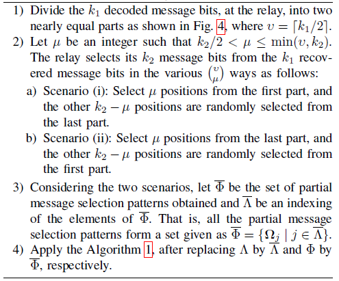
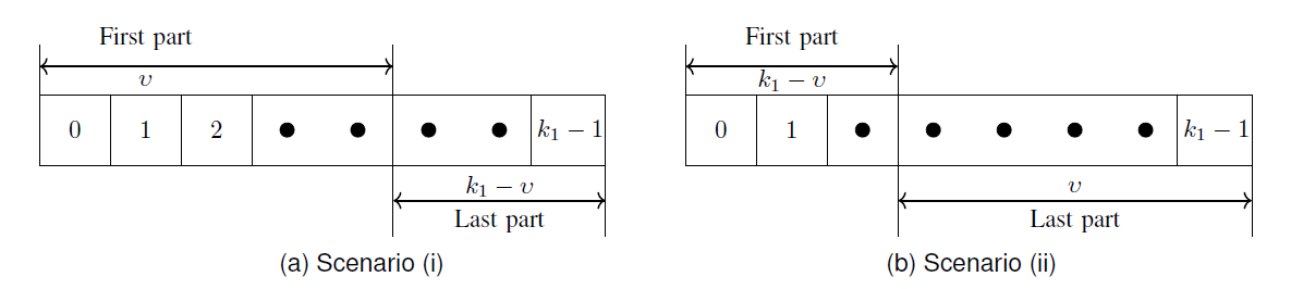
In general, the partial search procedure entails a division strategy at the relay for dividing the [TeX:] $$k_1$$ decoded message bits into two nearly equal parts and two scenarios, as illustrated in Fig. 4. Algorithm 2 summarizes the specific steps of the partial search method. We will refer to a design at the relay by Algorithms 1 and 2 as optimal and sub-optimal, respectively. A randomly designed relay channel code is one in which the selected bits patterns are drawn at random from both the message and parity bits of the decoded codeword [TeX:] $$\hat{\mathbf{c}}_1 \in C_S$$, and it is never empirically optimal or sub-optimal.
C. Complexity Analysis for the Two Relay Optimization Methods
In order to achieve the optimum destination codebook [TeX:] $$C_D^{(j)}$$ with respect to the largest free distance and improved spectrum, the relay must choose the best pattern [TeX:] $$\Omega_j$$ during the cooperation phase.
In the exhaustive search method, we apply Algorithm 1 to all [TeX:] $$\varphi=|\Phi|$$ codebooks where
(11)
[TeX:] $$|\Phi|=\left(\begin{array}{l} k_1 \\ k_2 \end{array}\right)=\frac{k_{1} !}{k_{2} !\left(k_1-k_2\right) !}.$$Since the factorial function, i.e., [TeX:] $$f(n)=n !$$ increase asymptotically with the value of n, then except for short codes, or values of [TeX:] $$k_2$$ very close to those of [TeX:] $$k_1$$, [TeX:] $$\varphi$$ is a very large number. The partial search approach, on the other hand, apply Algorithm 1 to [TeX:] $$\bar{\varphi}=|\bar{\Phi}|$$ codebooks where
[TeX:] $$v=\left\lceil k_1 / 2\right\rceil, \text { and } k_2 / 2\lt \mu \leq \min \left(v, k_2\right) \text {. }$$ This method, in particular, produces results where the difference between the values of [TeX:] $$v \text { and } \mu$$ is much smaller than the difference in the values of [TeX:] $$k_1$$ and [TeX:] $$k_2$$. Hence, [TeX:] $$\bar{\varphi}\lt\lt\varphi .$$
To encode one message of block length [TeX:] $$k_1$$ using a generator matrix [TeX:] $$\mathbf{G}_S$$ of size [TeX:] $$k_1 \times n$$ at the source, the number of multiplication operations performed is [TeX:] $$O_s^{\times}=k_1 n$$, and the number of addition operations is [TeX:] $$O_s^{+}=\left(k_1-1\right) n$$. Hence, a total of [TeX:] $$O_s^{\times}+O_s^{+}=k_1 n+\left(k_1-1\right) n$$ elementary operations are involved in encoding one message block. The number of elementary operations then becomes
for message blocks encoded by the source. Similarly, the total number of elementary operations required to encode message blocks retransmitted by the relay node is
In the destination’s view, [TeX:] $$\Gamma n$$ direct sum operations of the two codewords generated by the source and relay are performed. Hence, the total number of elementary operations performed for each unique jth selection pattern [TeX:] $$\Omega_j$$ fixed at the relay is
Consequently,
elementary operations are carried out in the exhaustive search method for [TeX:] $$\varphi$$ different selection patterns that are successively fixed at the relay. The number of elementary operations carried out in the partial search method is
for [TeX:] $$\bar{\varphi}$$ distinct selection patterns that are successively fixed at the relay. We obtain [TeX:] $$O^{\bar{\varphi}} \lt\lt O^{\varphi}$$.
V. JOINT DECODING
We designate by [TeX:] $$C_S \text {-decoder and } C_R \text {-decoder }$$ the decoders related to the TDCG codes employed by the source and relay, respectively. Each decoder will utilize the maximum likelihood decoding algorithm.
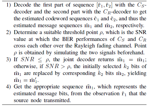
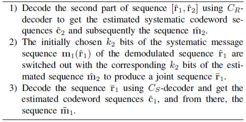
We employ a joint decoding scheme based on two different algorithms, namely, the naive Algorithm 3 and smart Algorithm 4. In contrast to the naive algorithm, smart algorithm always fully exploits the resources at the destination from each time slot of the coded-cooperation. In every joint decoding scheme, the two decoders, [TeX:] $$C_S \text {-decoder and } C_R \text {-decoder }$$, will be applied at the destination to decode the two parts of noisecorrupted compound codeword [TeX:] $$\left[\hat{\mathbf{r}}_1, \hat{\mathbf{r}}_2\right]$$ jointly constructed by the source and relay, respectively.
TABLE V
| Scheme | Selection Type | Selection pattern |
|---|---|---|
| [TeX:] $$M_1$$ | Optimal | [0, 1, 3] |
| Sub-optimal | [1, 2, 4] | |
| Random | [0, 1, 2] | |
| [TeX:] $$M_2$$ | Optimal | [2, 3, 4, 5, 6, 7, 8, 9, 10, 11, 13] |
| Sub-optimal | [0, 2, 3, 4, 5, 6, 7, 8, 9, 10, 11] | |
| Random | [0, 1, 2, 3, 4, 5, 6, 7, 10, 11,12] | |
| [TeX:] $$M_3$$ | Sub-optimal | [0, 2, 3, 4, 5, 6, 7, 8, 9, 11, 12, 13, 14, 15, 16, 17, 18, 19] |
| Random | [0, 1, 2, 3, 4, 5, 6, 7, 8, 9, 10, 11, 12, 13, 14, 15, 16, 17] |
VI. ERROR PERFORMANCE COMPARISONS FOR VARIOUS SCHEMES
This section examines the bit-error-rate (BER) performances of the TDCGCC schemes in a flat fading channel under various channel conditions. The numerical simulation analysis has considered the TDCGCC schemes listed in Table II. Each TDCGCC system employs BPSK modulation with coherent detection over a fast Rayleigh fading channel. We represent the SNR for the channel between the (S-D), (S-R), and (R-D) links, respectively, by the symbols [TeX:] $$\lambda_{S, D}, \lambda_{S, R} \text {, and } \lambda_{R, D}$$. The total energy of each transmission scheme is taken to be unity. Each corresponding receiver has complete knowledge of the channel state. The relay always achieves SNR gain over the source because it is closer to the source than the destination is to the source. It is also assumed that [TeX:] $$\lambda_{R, D}=\lambda_{S, D}+2 \mathrm{~dB}$$
A. BER Performance of TDCGCC Scheme under Different Designed Relay Channel Codes
Fig. 5.
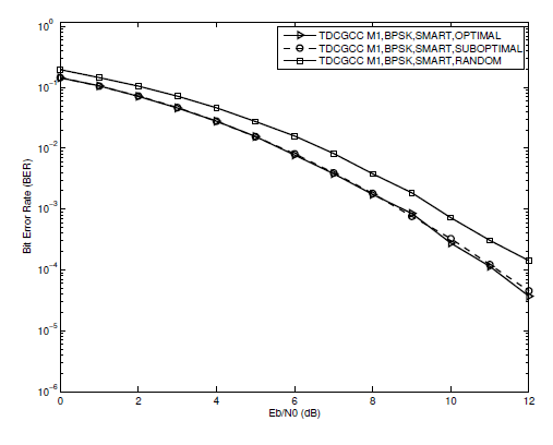
Fig. 6.
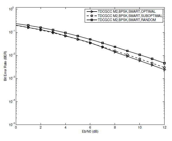
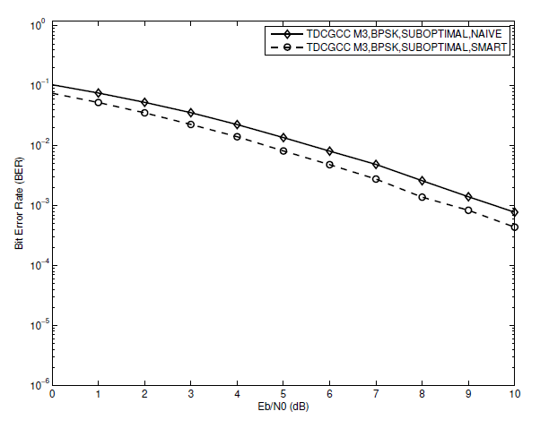
A performance comparison between optimized (i.e., optimal and sub-optimal) and un-optimized (i.e., random) designed relays in each TDCGCC scheme is investigated in this section. For a fair comparison, (S-R) link is assumed to be ideal, i.e., [TeX:] $$\left(\lambda_{S, R}=\infty\right)$$, and the joint decoder employs the smart algorithm. First, we look at the simulation results of the TDCGCC schemes [TeX:] $$M_1 \text { and } M_2$$ with both optimal and suboptimal relay designs plotted in Figs. 5 and 6, respectively. Both optimal and sub-optimal relay designs yield nearly the same BER performance at low to medium SNR, while at high SNR, the TDCGCC schemes with optimally designed relay nodes slightly outperform ones with the sub-optimally designed relay nodes. Since the sub-optimal design of a relay has a reduced processing complexity, it is then suggested and adopted for optimizing the TDCGCC schemes in all subsequent performance analyses.
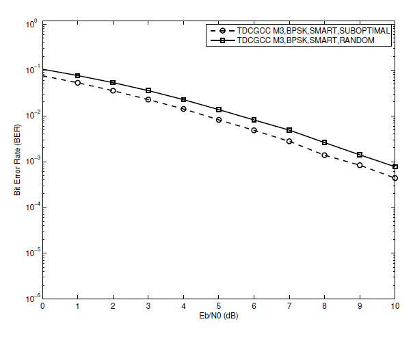
Secondly, we look at the simulation results of the TDCGCC schemes [TeX:] $$M_1, M_2, \text { and } M_3$$ with un-optimized (i.e., random) and optimized (i.e., sub-optimal) designed relay designs plotted in Figs. 5, 6, and 7, respectively. The un-optimized designed relay lags behind the optimized designed relay and continuously gets degraded with an increase in the SNR. Evidently, optimized design in the relay node greatly improves the overall performance of a TDCG coding scheme. The loss in the BER performance of un-optimized design channel code is attributable to improper bit selection at the relay, which reduces the cooperation resources and hence the overall system performance.
B. BER Performance of TDCGCC Schemes Employing Naive and Smart Joint Decoding Algorithms
Fig. 8.
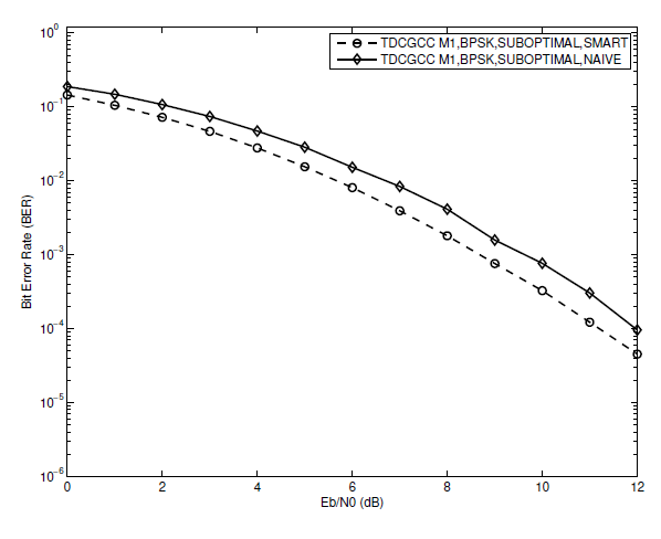
Fig. 9.
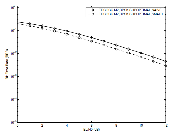
Fig. 10.
We should use a decoding approach that can make use of all the resources that our optimized relay channel has to offer. For each of the three schemes [TeX:] $$M_1, M_2, \text { and } M_3$$, two decoding strategies the Naive Algorithm 3 and Smart Algorithm 4 joint decoding algorithms-are compared.We assume that each of the schemes uses an ideal (S-R) link and a sub-optimal designed relay. Figs. 8, 9, and 10 display the results from the Monte Carlos simulation. When the joint decoder uses the smart algorithm instead of the naive algorithm, the BER performance is better for each of the three TDCGCC schemes. This is due to the fact that the smart algorithm gains an advantage by feeding more reliable CR-decoder decoded bits into the CS-decoder during the joint decoding. For instance, utilizing the smart algorithm schemes [TeX:] $$M_1, M_2, \text { and } M_3$$, respectively, outperforms the naive algorithm scheme by approximately 0:8 dB, 1 dB, and 1:1 dB each at the [TeX:] $$\mathrm{BER}=10^{-2}$$, as shown in Figs. 8, 9, and 10, respectively. These results demonstrate the value of resources made available through optimized cooperation.
C. BER Performance Comparison of TDCGCC Schemes with their Corresponding Non-cooperative Counterparts
Fig. 11.
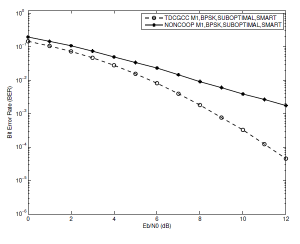
Fig. 12.
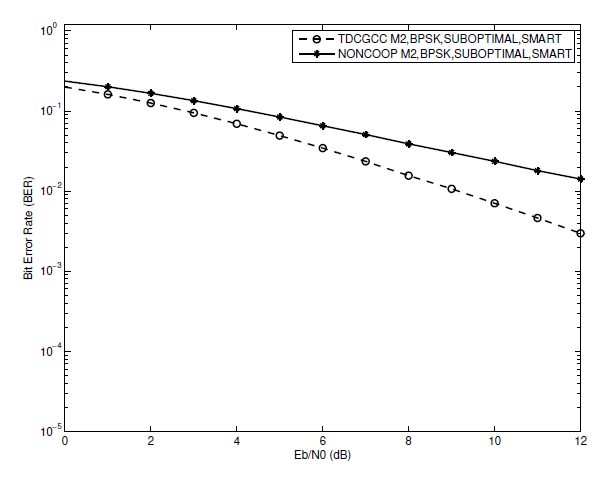
Fig. 13.
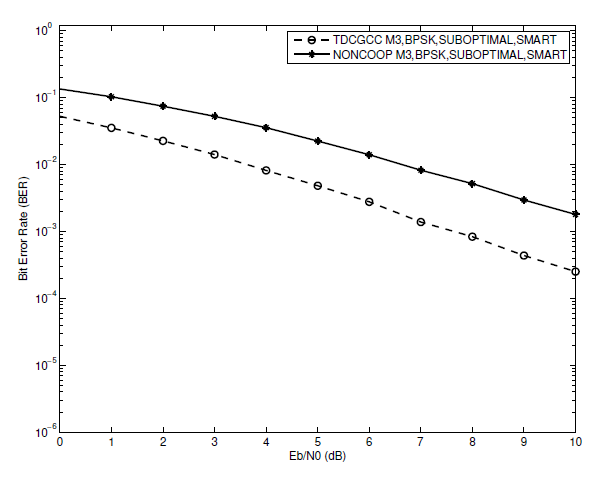
In the preceding simulation results in Sections VI-A and VI-B, the best conditions for a TDCGCC scheme to achieve full diversity are illustrated. These include a perfect (S-R) link, joint decoding based on a smart algorithm, and optimized relay channel code design. When comparing the BER performance of the non-cooperative (direct link) system and the TDCGCC scheme, we make use of these best conditions. Cooperation leads to improvements, as shown in Figs. 11, 12, and 13. Scheme [TeX:] $$M_1$$ has a 1:9 dB gain, for instance, when has a 1:9 dB gain, for instance, when [TeX:] $$\mathrm{BER}=1 \times 10^{-2}.$$ Scheme [TeX:] $$M_2$$ gain is approximately 2:7 dB at [TeX:] $$\mathrm{BER}=1.1 \times 10^{-2}$$, while Scheme [TeX:] $$M_3$$ gain is roughly 3 dB at [TeX:] $$\mathrm{BER}=1 \times 10^{-2}$$. We observe that the TDCGCC schemes post impressive performance as compared with corresponding noncooperative counterparts. These results validates the efficacy of the proposed TDCGCC scheme.
D. BER Performance of TDCGCC Scheme over Practical (Non-Ideal) and Ideal Source-to-Relay Channels
Fig. 14.
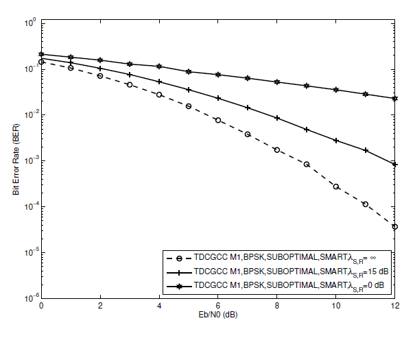
Fig. 15.
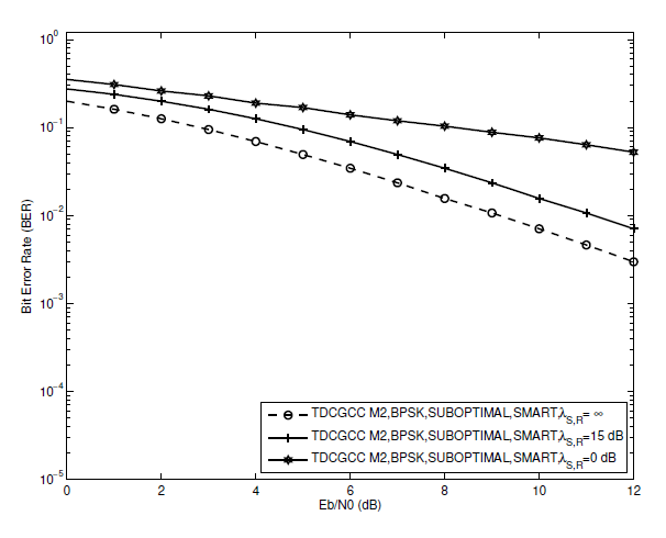
Fig. 16.
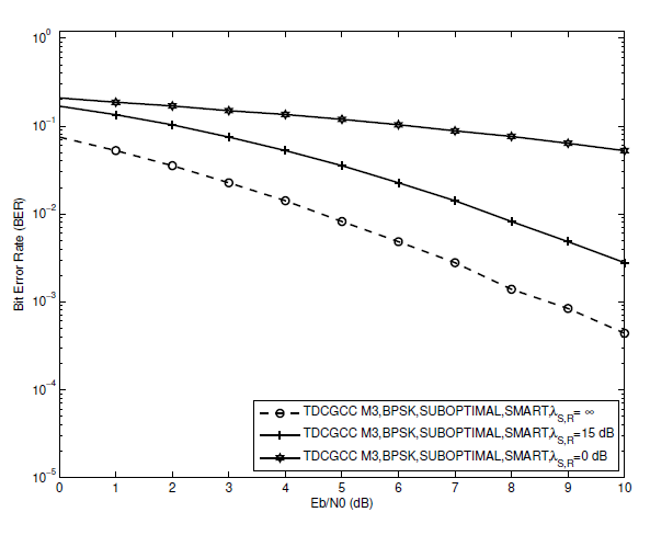
The perfect (S-R) channel, i.e., [TeX:] $$\lambda_{S, R}=\infty$$, is not possible for the majority of real-world applications. The following presumptions are made to evaluate the performance of each of the three TDCGCC schemes in such situations. We choose to set the non-ideal channel circumstances to either a poor (S-R) link, let’s say [TeX:] $$\lambda_{S, R}=0 \mathrm{~dB}$$, or a good (S-R) link, let’s say [TeX:] $$\lambda_{S, R}=15 \mathrm{~dB}$$. We also assume that no additional error propagation mitigation techniques, such as those proposed in [3], [30], are used at the relay and that the relay always takes part in the coded cooperation regardless of whether the relay terminal’s decoding is accurate or not. Fig. 14 shows that at [TeX:] $$\mathrm{BER}=1 \times 10^{-3}$$, the TDCGCC scheme [TeX:] $$M_1$$ with a (S-R) link of [TeX:] $$\lambda_{S, R}=15 \mathrm{~dB}$$ is only behind the ideal (S-R) link by about 2:2 dB. Similar results can be seen in Figs. 15 and 16, where the TDCGCC schemes under (S-R) link of [TeX:] $$\lambda_{S, R}=15 \mathrm{~dB}$$ are only 1:8 dB and 2:6 dB worse than that under the ideal (S-R) link at [TeX:] $$\mathrm{BER}=1 \times 10^{-2}$$ correspondingly. Therefore, the TDCGCC scheme performance approaches that of an ideal link when the (S-R) link become excellent.
However, the BER performance of TDCGCC schemes is severely hampered if the (S-R) link deteriorates, let’s say to [TeX:] $$\lambda_{S, R}=0 \mathrm{~dB}$$. Figs. 14, 15, and 16 demonstrate this, where the BER curves become practically flat at the (S-R) link of [TeX:] $$\lambda_{S, R}=0 \mathrm{~dB}$$. The relay node is unable to perform an accurate decoding due to the poor channel state between the source and relay nodes. As a result of the propagation of errors from the relay node, the destination node is unable to perform accurate joint-decoding, which lowers overall BER performance.
E. BER Performance of TDCGCC in Comparison to BCH Coded-cooperative Scheme and Other Existing Coded Cooperation Methods of Similar Rates
The Goppa code is a subfield subcode of a GRS code, just like the BCH code [31] is a subfield subcode of a RS code. Since their theory and application are reasonably simple, BCH codes are the most used in practice. Both codes are two most important subclasses of a broad class of Alternant codes [14]. BCH codes are well-known for performing well at short lengths, outperforming other codes including LDPC, RM, and polar codes [32]. As a fair comparison, first, we measure the TDCG code’s performance against a binary BCH code with a comparable length and code rate. The parameters of the BCH codes, which are used in schemes [TeX:] $$M_4, M_5, \text { and } M_6$$ to compare with TDCG codes in schemes [TeX:] $$M_1, M_2, \text { and } M_3$$, are described in Table VI. Since the BCH code only has one extra information bit than the comparable TDCG code, we assume the difference in data rates is negligible. Table VII lists the selection patterns associated to the various BCH coded-cooperative (BCHCC) schemes. Next, we present a BER performance comparison between the TDCGCC and the existing coded cooperation methods referenced. We have considered the following coded cooperation methods. RM codes, which employ [TeX:] $$C_S=R M(2,4) \text { and } C_R=R M(1,4),$$ and overall system rate of 11/32 [33], RS coded cooperation with adaptive cooperation level scheme with an overall system rate of 2/5 [6], and network-turbo code based distributed space-time block code (DSTBC-NTC) cooperative scheme with an overall system rate of 1/3 [34]. As such, we compare them with the TDCGCC scheme [TeX:] $$M_2$$, which has a similar overall system rate of 14/42.
TABLE VI
| Scheme Serial | [TeX:] $$C_S\left(n_1, k_1, d_1\right)$$ | [TeX:] $$C_R\left(n_2, k_2, d_2\right)$$ | [TeX:] $$C_D\left(n_1+n_2, k_1\right)$$ | [TeX:] $$d_{\text {free }}$$ | Rate (R) |
|---|---|---|---|---|---|
| [TeX:] $$M_4$$ | [21,6,7] | [21,4,9] | [42, 6] | 7 | 0.1429 |
| [TeX:] $$M_5$$ | [21,15,3] | [21,12,5] | [42, 15] | 3 | 0.3571 |
| [TeX:] $$M_6$$ | [73,28,17] | [73,19,21] | [146,28] | 17 | 0.1918 |
TABLE VII
| Scheme | Selection Type | Selection Pattern |
|---|---|---|
| [TeX:] $$M_4$$ | Sub-optimal | [0, 2, 3, 4] |
| [TeX:] $$M_5$$ | Sub-optimal | [0, 1, 2, 3, 4, 5, 6, 8, 9, 12, 13, 14] |
| [TeX:] $$M_6$$ | Sub-optimal | 0, 1, 3, 5, 6, 7, 9, 10, 11, 12, 13, 14, 15, 16, 17, 18, 19, 20, 21] |
Fig. 17.
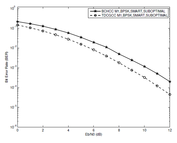
Fig. 18.
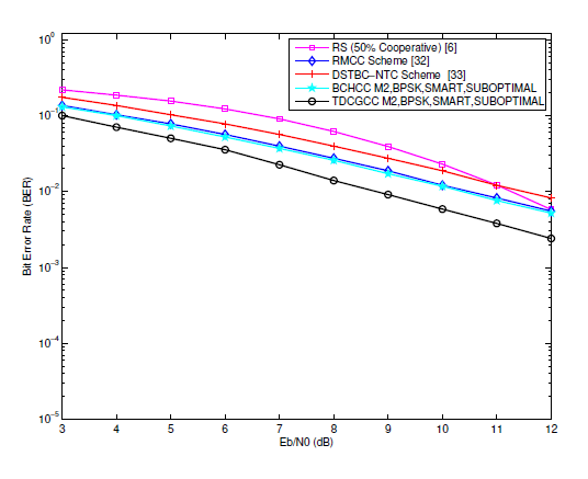
Fig. 19.
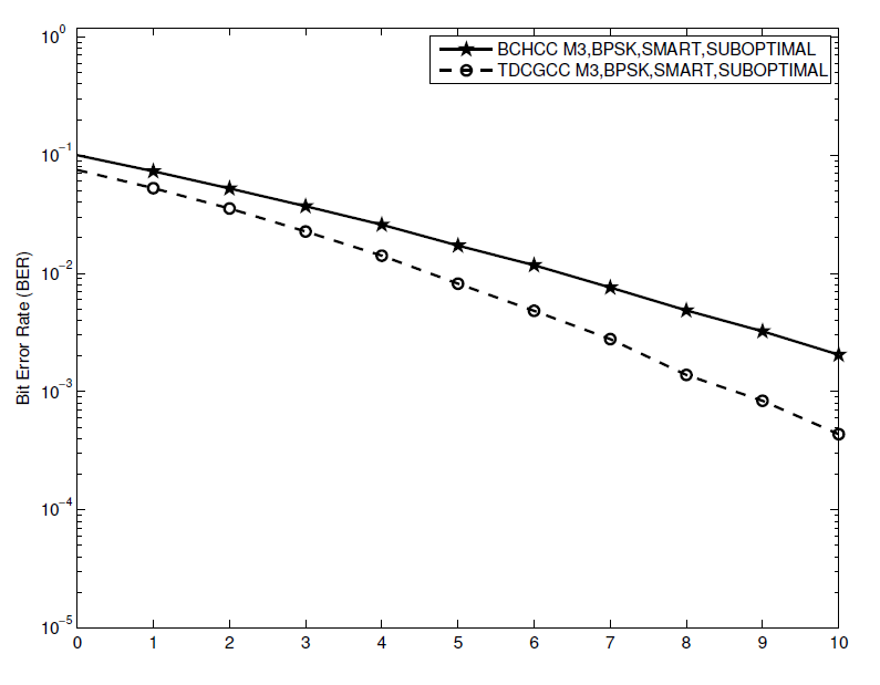
Figs. 17, 18, and 19 show that, at [TeX:] $$\mathrm{BER}=1 \times 10^{-2}$$, the TDCGCC schemes [TeX:] $$M_1, M_2, \text { and } M_3$$ perform better than the BCHCC schemes [TeX:] $$M_4, M_5, \text { and } M_6$$, respectively, by about 1.1 dB, 0.8 dB, and 1.7 dB. Despite having one less information bit, a TDCGCC scheme offers a substantial advantage over a BCHCC scheme of a similar overall system rate. This enticing advantage can be attributed to the TDCG codes used at the source and relay nodes having a noticeably greater minimum Hamming distance, i.e., they have parameter such as those of the best-known linear codes. Therefore, when utilized in coded-cooperative coding schemes, TDCG codes remain to be superior to binary BCH codes.
The simulation results, which are also presented in Fig. 18, show how the proposed TDCGCC scheme outperforms existing ones like the RMCC in [33], the RS adaptive scheme (50% cooperative) in [6], and the DSTBC-NTC cooperative scheme in [34]. In comparison to the RMCC, RS adaptive (50% cooperative), and DSTBC-NTC cooperative schemes, the TDCGCC scheme, for instance, achieves improvements of around 0.9 dB, 2.5 dB and 2.8 dB at [TeX:] $$\mathrm{BER} \approx 1 \times 10^{-2}$$, respectively.
VII. CONCLUSION
The main goal of the research is to investigate a novel induced-cyclic TDCG coded-cooperative diversity scheme. Since TDCG codes are among the best-known linear codes, they produce an excellent coded-cooperative system. The relay channel code is optimized using an effective method, which is shown to improve system performance. The simulation results showed that, when using joint decoding based on the smart algorithm and with an optimized relay, the TDCGCC scheme outperforms the non-cooperative method with outstanding results. The two factors that account for the TDCGCC schemes’ impressive performance are the joint decoding carried out at the destination, which successfully recovers the information from the source, and the added SNR gain provided by the optimized relay. Indeed, numerical simulation findings demonstrate that the proposed TDCGCC scheme performs better than the BCHCC and other existing coded-cooperation methods using the RM, RS, and DSTBC-NTC codes.
Biography
Daniel Kariuki Waweru
Daniel Kariuki Waweru received his B.Sc. degree in Mathematics and M.Sc. degree in Pure Mathematics from the University of Nairobi, Kenya, in 2015 and 2017, respectively. He is currently doing a Ph.D. from the College of Electronic and Information Engineering, Nanjing University of Aeronautics and Astronautics, China. His main interest is in algebraic coding theory, especially in the connections between codes, algebraic geometry and computer algebra tools. His most recent work are concerned with algebra-geometric codes and their application in wireless communications.
Biography
Fengfan Yang
Fengfan Yang received the M.Sc. and Ph.D. degrees from the Northwestern Polytechnical University and Southeast University, China in 1993, and 1997, respectively, all in Electronic Engineering. Presently, he is working as a Professor in the College of Electronic and Information Engineering, Nanjing University of Aeronautics and Astronautics, China. His major research interests are information theory, channel coding and their applications for mobile and satellite communications.
Biography
Chunli Zhao

Chunli Zhao received her B.S. degree in Electronic and Information Engineering from Henan Normal University Xinlian College, China, in 2014. She obtained her M.Sc. degree in Circuits and Systems at Henan Normal University, China, in 2017. She is currently doing a Ph.D. from the College of Electronic and Information Engineering, Nanjing University of Aeronautics and Astronautics, China. Her research interests are circuits and systems, signal processing, and channel coding.
Biography
Lawrence Muthama Paul
Lawrence Muthama Paul obtained a B.Sc. degree in Mathematics in September, 2017 from the University of Nairobi, Kenya, and M.Sc. degree in Pure Mathematics in September, 2019 from the same University. From September, 2019 to September, 2020, he was a Graduate Assistant at the University of Nairobi. Currently, he is a Doctoral Student in the College of Electronic and Information Engineering, Nanjing University of Aeronautics and Astronautics, China. His current research interests are in algebra geometry coding theory and its applications in wireless communication.
References
- 1 A. Sendonaris, E. Erkip, and B. Aazhang, "User cooperation diversity part I: System description," IEEE Trans. Commun., vol. 51, no. 11, pp. 1927-1938, Nov. 2003.doi:[[[10.1109/TCOMM.2003.818096]]]
- 2 J. N. Laneman, G. W. Wornell, and D. N. Tse, "An efficient protocol for realizing cooperative diversity in wireless networks," in Proc. IEEE ISIT, 2001.doi:[[[10.1109/isit.2001.936157]]]
- 3 T.E. Hunter and A. Nosratinia, "Diversity through coded cooperation," IEEE Trans. Wireless Commun., vol. 5, no. 2, pp. 283-289, Feb. 2006.doi:[[[10.1109/twc.2006.1611050]]]
- 4 Y . Fang, S. C. Liew, and T. Wang, "Design of distributed protograph LDPC codes for multi-relay coded cooperative networks," IEEE Trans. Wireless Commun., vol. 16, no. 11, pp. 7235-7251, Aug. 2017.doi:[[[10.1109/TWC.2017.2743699]]]
- 5 S. Ejaz and F. Yang, "Jointly optimized Reed-Muller codes for multilevel multi relay coded-cooperative V ANETS," IEEE Trans. Veh. Technol., vol. 66, no. 5, pp. 4017-4028, Aug. 2017.doi:[[[10.1109/TVT.2016.2604320]]]
- 6 A. H. M. Almawgani and M. F. M. Salleh, "RS coded cooperation with adaptive cooperation level scheme over multipath rayleigh fading," in Proc. IEEE ICC, 2009.doi:[[[10.1109/MICC.2009.5431555]]]
- 7 J. Qiu, L. Chen, and S. Liu, "A novel concatenated coding scheme: RSSC-LDPC codes," IEEE Commun. Lett., vol. 24, no. 10, pp. 2092-2095, Oct. 2020.custom:[[[http://www.chencode.cn/publications/j_papers/qiujie2020.pdf]]]
- 8 S. Mughal, F. Yang, and S. Ejaz, "Asymmetric turbo code for codedcooperative wireless communication based on matched interleaver with channel estimation and multi-receive antennas at the destination," Radioengineering, vol. 26, no. 3, pp. 878-889, Sep. 2017.doi:[[[10.13164/re.2017.0878]]]
- 9 S. Ejaz and F.-F. Yang, "Turbo codes with modified code matched interleaver for coded-cooperation in half-duplex wireless relay networks," Frequenz, vol. 69, no. 3-4, pp. 171-184, Mar. 2015.doi:[[[10.1515/freq-2014-0072]]]
- 10 R. Umar, F. Yang, and H. J. Xu, "Multilevel construction of polar-coded single carrier-FDMA based on MIMO antennas for coded cooperative wireless communication," IET Commun., vol. 12, no. 10, pp. 1253-1262, Jun. 2018.doi:[[[10.1049/iet-com.2017.1436]]]
- 11 Q. Zhan, D. Minghui, Y . Wang, and F. Zhou, "Half-duplex relay systems based on polar codes," IET Commun., vol. 8, no. 4, pp. 433-440, Mar. 2014.doi:[[[10.1049/iet-com.2013.0521]]]
- 12 R. Blasco-Serrano, R. Thobaben, M. Andersson, V . Rathi, and M. Skoglund, "Polar codes for cooperative relaying," IEEE Trans. Commun., vol. 60, no. 11, pp. 433-440, Aug. 2012.doi:[[[10.1109/TCOMM.2012.081412.110266]]]
- 13 J.G. Proakis and M. Salehi, Digital Communications. McGraw-Hill, 2008.doi:[[[10.1007/978-1-4939-7393-4_6]]]
- 14 F.J. MacWilliams and N.J.A. Sloane, The Theory of Error-Correcting Codes, vol. 16, page iii, Elsevier, 1977.custom:[[[https://www.elsevier.com/books/the-theory-of-error-correcting-codes/macwilliams/978-0-444-85193-2]]]
- 15 V .D. Goppa, "A new class of linear error-correcting codes," Problemy Peredachi Informatsii, vol. 6, no. 3, pp. 24-30, 1970.custom:[[[-]]]
- 16 V .D. Goppa, "Rational representation of codes and (L,g)-codes," Problems Inf. Transmission, vol. 7, no. 3, pp. 41-49, 1971.custom:[[[https://www.mathnet.ru/php/archive.phtml?wshow=paper&jrnid=ppi&paperid=1647&option_lang=eng]]]
- 17 C. Moreno, Algebraic curves over finite fields, in Cambridge Tracts in Mathematics 97. Cambridge Univ. Press, Cambridge, U.K., 1991.doi:[[[10.1017/cbo9780511608766]]]
- 18 M.A. Tsfasman, S.G. Vladut, and T. Zink, "On Goppa codes which are better than the Varshamov-Gilbert bound," Mathematische Nachrichten, vol. 109, pp. 21-28, 1982.custom:[[[https://www.mathnet.ru/php/archive.phtml?wshow=paper&jrnid=ppi&paperid=1231&option_lang=eng]]]
- 19 M. Grass, Bounds on the minimum distance of linear codes and quatum codes. (Online). Available: http://www.codetables.decustom:[[[http://www.codetables.de]]]
- 20 Y . Sugiyama, M. Kasahara, S. Hirasawa, and T. Namekawa, "A method for solving key equation for decoding Goppa codes," Inf. Control, vol. 27, no. 1, pp. 87-99, Jan. 1975.doi:[[[10.1016/s0019-9958(75)90090-x]]]
- 21 Y . Sugiyama, M. Kasahara, S. Hirasawa, and T. Namekawa, "Further results on goppa codes and their applications to constructing efficient binary codes," IEEE Trans. Inf. Theory, vol. 22, no. 5, pp. 518-526, Sep. 1976.doi:[[[10.1109/TIT.1976.1055610]]]
- 22 S. Bezzateev and N. Shekhunova, "Totally decomposed cumulative Goppa codes with improved estimations," Designs, Codes Cryptography, vol. 87, pp. 569-587, Mar. 2019.doi:[[[10.1007/s10623-018-0566-2]]]
- 23 T. P. Berger, "On the cyclicity of Goppa codes, parity-check subcodes of Goppa codes and extended Goppa codes," Finite Fields Applications, vol. 6, no. 3, pp. 255-281, Jul. 2000.doi:[[[10.1006/ffta.2000.0277]]]
- 24 S. V . Bezzateev and N. A. Shekhunova, "Subclass of cyclic Goppa codes," IEEE Trans. Inf. Theory, vol. 59, no. 11, pp. 7379-7385, Aug. 2013.doi:[[[10.1109/tit.2013.2278176]]]
- 25 K. K. Tzeng and K. Zimmermann, "On extending Goppa codes to cyclic codes,". IEEE Trans. Inf. Theory, vol. 21, pp. 712-716, Nov. 1975.doi:[[[10.1109/TIT.1975.1055449]]]
- 26 T. P. Berger, "Cyclic alternant codes induced by an automorphism of a GRS code," Finite Fields: Theory, Applications and Algorithms, vol. 225, 1999.doi:[[[10.1090/conm/225/03216]]]
- 27 F. Ghavimi and H.-H. Chen, "M2m communications in 3gpp lte/lte-a networks: Architectures, service requirements, challenges, and applications," IEEE Comm. Surveys Tuts., vol. 17, no. 2, pp. 525-549, Oct. 2015.doi:[[[10.1109/comst.2014.2361626]]]
- 28 Z. Ding et al., "A survey on non-orthogonal multiple access for 5G networks: Research challenges and future trends," IEEE J. Sel. Areas Commun., vol. 35, no. 10, pp. 2181-2195, Jul. 2017.doi:[[[10.1109/jsac.2017.2725519]]]
- 29 E. C. Van Der Meulen, "Three-terminal communication channels," Advances Appl. Probability, vol. 3, no. 1, pp. 120-154, 1971.doi:[[[10.1017/s0001867800037605]]]
- 30 T. Van Nguyen, A. Nosratinia, and D. Divsalar, "Bilayer protograph codes for half-duplex relay channels," IEEE Trans. Wireless Commun., vol. 12, no. 5, pp. 1969-1977, Apr. 2013.doi:[[[10.1109/isit.2010.5513451]]]
- 31 R.C. Bose and D.K. Ray-Chaudhuri, "On a class of error correcting binary group codes," Inf. Control, vol. 3, no. 1, pp. 68-79, Mar. 1960.doi:[[[10.1016/s0019-9958(60)90287-4]]]
- 32 J. Van Wonterghem, A. Alloum, J.J. Boutros, and M. Moeneclaey, "Performance comparison of short-length error-correcting codes," in Proc. SCVT, 2016.doi:[[[10.1109/scvt.2016.7797660]]]
- 33 S. Ejaz, F. Yang, and H. Xu, "Jointly optimized multiple Reed-Muller codes for wireless half-duplex coded-cooperative network with joint decoding," EURASIP J. Wireless Commun. Netw., vol. 2015, pp. 1-15, Dec. 2015.doi:[[[10.1186/s13638-015-0334-1]]]
- 34 B. Chen and M. Flanagan, "Network-turbo-coding based cooperation with distributed space-time block codes," Trans. Emerging Telecommun. Technol., vol. 26, no. 6, pp. 992-1002, Jun. 2015.custom:[[[https://ieeexplore.ieee.org/document/6582794]]]