Seong Ho Chae , Hyeongyong Lim , Howon Lee and Bang Chul Jung
Performance Analysis of Dense Low Earth Orbit Satellite Communication Networks with Stochastic Geometry
Abstract: The low Earth orbit (LEO) satellite communication systems have drawn much attention as a promising solution for providing global wireless connectivity. This paper studies the downlink performances of LEO satellite communication systems performing a directional beamforming with a stochastic geometry. As the beamwidth of the satellite increases, the beam coverage increases but the interference from other satellites also increases. This is vice versa for the smaller beamwidth. Accordingly, the optimal beamwidth control is necessary to balance the beam coverage and the network interference. To address such issue, we first derive the conditional distance distribution to serving line-of-sight (LoS) and non-line-of-sight (NLoS) satellites, conditioned on that there exists at least one satellite in the satellite-visible region and the user is located within the beam coverage of the satellite. Then, we derive the exact and approximated formulas for the coverage probability and the ergodic rate as a function of the beamdwidth. With some numerical examples, we investigate how various system parameters such as altitude and satellite density affect on the optimal beamwidth and demonstrate that the optimal control of the beamwidth of the satellites can maximize the performances by efficiently controlling the amount of interference and beam coverage.
Keywords: Coverage probability , ergodic rate , satellites , stochastic geometry
I. INTRODUCTION
THE recent rapid development of mobile devices and datahungry multimedia applications have triggered users’ unprecedented increasing demands for high data-rate and ubiquitous connectivity. To meet such ever-increasing demands, the new communication technologies and network designs have been being developed for the terrestrial networks. However, high construction cost of network facilities and physical infrastructure deployment constraints make the terrestrial networks being still unavailable in many less-developed areas or low population density areas. Accordingly, the network operators meet new challenges to develop novel solutions for providing ubiquitous connectivity everywhere around the world.
With the recent space launch cost reduction and the development of advanced launch system, the satellites have drawn much attention as a promising solution to provide the wireless global coverage. Particularly, the low Earth orbit (LEO) satellites have gained increasing interests in both academy and industry because they are deployed at a relatively low altitude of 500–1500 km above the ground and offer the several advantages such as low pathloss, low propagation delay, cheaper launching cost, low energy consumption, high-throughput, and low-cost internet access [1], [2]. Indeed, various industrial companies, such as SpaceX, Amazon, OneWeb, Google, and Telesat, have announced plans to launch thousands of LEO satellites for providing wireless global coverage [3]. Specifically, Starlink, Project Kuiper, Telesat LEO, have a plan to launch LEO satellites of 42,000, 3,236, and 512, respectively [4], [5]. Many other companies and governments also have plans to deploy dense small satellite networks, so it is expected that the satellite networks may become more and more dense and complex.
Recently, there have been growing interests in the design and optimization of satellite communication networks and various advanced techniques to improve the performances have been developed [6]–[12]. The non-orthogonal multiple access (NOMA) scheme was proposed for satellite network and its outage probability and diversity order were investigated over Shadowed-Rician fading channel [6]. Various graph based handover algorithms to maximize the benefits of mobile terminals and balance the loads were proposed in [7]–[9]. The massive MIMO technique with full frequency reuse scheme was proposed for LEO satellite communication networks [10]. The heuristic beam shut off algorithm to minimize the number of active beams was proposed in LEO multibeam satellite networks [11] and the Stackelberg game based cache resource allocation to balance the loads was proposed in multi-layers satellite networks [12]. However, these techniques were developed for a small number of satellites, so the effects of the large number of satellites such as interference were not well characterized.
The conventional model to study the performances of satellite networks is a regular deterministic model, where all satellites are evenly spaced with the same period and the inclination [13]. However, this model requires the extensive system level-simulations, which makes hard to get useful design insights with a tractable form. The stochastic geometry has been deemed as a useful mathematical tool to analyze the network performance with a tractable form and there have recently been some trials to understand the fundamentals of the satellite communication networks with stochastic geometry [14]–[23]. In [14], the coverage probability of downlink multi-beam satellite communication network was investigated in which a single satellite serves multiple users via multi spot beams with the random user selection and the best user selection. The cumulative distribution function of the nearest neighbor distance for the multiple concentric spheres model was studied in [15]. The coverage and outage probabilities of the LEO satellite networks were analyzed with a binomial point process (BPP) model over Shadowed-Rician fading channel [16], [17], but these works did not characterize the interferences from other satellites. The coverage probability and average rate of downlink LEO satellite networks were analyzed with a BPP over Rayleigh fading and non-fading in the presence of network interference [18]. The coverage probability of dense satellite networks was investigated with Poisson point process (PPP) model [19], but the explicit form was not provided. The coverage probability was analyzed with PPP over Nakagami-m fading channel, but the beamwidth control issue was not tackled and LoS/NLoS transmission model based interference effects were not well captured [20]. The coverage probability and average data rate of LEO network were analyzed with a non-homogeneous PPP model [21] and the optimal altitude of PPP based dense satellite constellations to maximize the coverage probability was investigated [22]. The algorithm to calculate the distance of different point sets was proposed and the distance between BPP and Fibonacci lattice/orbit models was compared in [23]. However, none of the above works have successfully analyzed the performances by considering the beamwidth control of directional beamforming, which is the main focus of this paper.
A. Contributions
The contributions of this paper are summarized as follows:
The spatial modeling of satellite communication networks is of great importance for their design and performance analysis. In the satellite communication networks performing a directional beamforming, as the beamwidth becomes wide, the beam coverage increases but the beam power gain decreases and the number of interfering satellites increases. On the contrary, as the beamwidth becomes narrow, the beam power gain increases and the number of interfering satellite decreases but the beam coverage decreases. Therefore, the optimal control of beamwidth is necessary to efficiently control the network interference and the beam coverage. To address such issue, we model the satellite communication networks with a stochastic geometry, where the satellites perform a directional beamforming of which transmit antenna gain is a function of beamwidth.
We newly derive the set of analytical results for signalto- interference-plus-noise ratio (SINR) for the satellite communication networks with a directional beamforming. Specifically, we derive the conditional probability distribution function (PDF) and conditional cumulative distribution function (CDF) of the distance to the serving line-of-sight (LoS) and non-line-of-sight (NLoS) satellite, conditioned on that there exists at least one satellite in the satellite-visible region and the user is located within the beam coverage of the satellite. We also derive the conditional Laplace transform of the aggregate interference conditioned on that the user is tagged on LoS or NLoS satellite. Using those statistics, we derive the exact analytical expressions for coverage probability and ergodic rate and their tractable approximated formulas.
Our numerical results demonstrate that the optimal control of the beamwidth of the satellites can maximize the performances by efficiently controlling the network interference and beam coverage. We discover that the optimal beamwidth for lower altitude is more larger than that for higher altitude and the optimal beamwidth decreases as the satellite density increases for maximizing the coverage probability. We also numerically investigate how various system parameters, such as Nakagami-m fading parameters, the pathloss exponents, the altitude, the zenith angle of LoS/NLoS transmission, and the satellite density, affect on the coverage probability and the ergodic rate.
B. Organizations
The rest of the paper is organized as follows. We describe the system model in Section II and analyze the coverage probability and average rate in Section III and Section IV, respectively. Numerical examples to validate our analysis are provided in Section V and the conclusion is drawn in Section VI.
II. SYSTEM MODEL
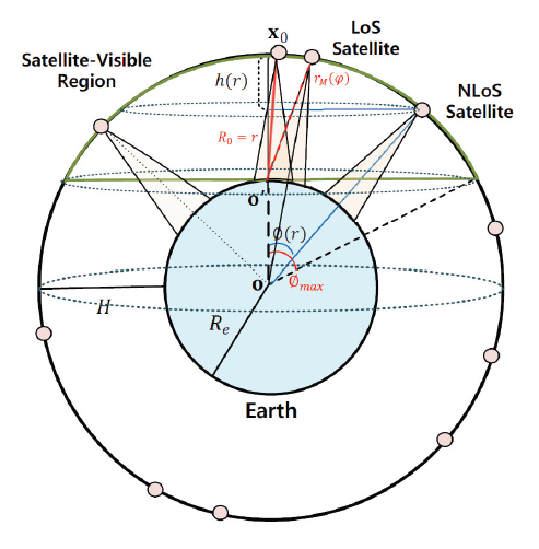
We consider the downlink dense satellite communication networks performing a directional beamforming, where the satellites are uniformly distributed over the Earth-centered spherical surface with altitude H [km] from the Earth and they communicate with users on the Earth. We call this spherical surface Earth orbit region in the rest of the paper. We assume that Earth is a sphere of a radius [TeX:] $$R_e(\sim 6,371[\mathrm{km}])$$ centered at the origin [TeX:] $$\mathbf{o} \triangleq(0,0,0) \in \mathbb{R}^3$$ in the 3D Cartesian coordinate system. Accordingly, the Earth orbit region can be regarded as the spherical surface of a radius [TeX:] $$R_e+H$$ centered at the origin. We model the satellites as a homogeneous PPP with intensity and denote the set of their locations as [TeX:] $$\Phi=\left\{\mathbf{x}_l\right\}$$, where [TeX:] $$\mathrm{x}_l \in \mathbb{R}^3$$ indicates the location of l-th satellite. We assume that the satellites employ an ideal directional beamforming which radiates the conical beam of beamwidth [TeX:] $$\varphi(\gt 0)$$ towards the center of the Earth. The transmit antenna beam gain can be represented by
(2)
[TeX:] $$G(\varphi)= \begin{cases}\min \left\{G_{\max }, \frac{1-\cos \left(\varphi_{\max } / 2\right)}{1-\cos (\varphi / 2)}\right\} \text { for }|\varphi| \leq \varphi_{\max }, \\ 0 \text { otherwise, }\end{cases}$$where [TeX:] $$\varphi_{\max }=\arccos \left(\frac{H^2+2 H R_e-R_e^2}{\left(R_e+H\right)^2}\right)$$ represents the maximum beamwidth which covers the entire earth surface and [TeX:] $$G_{\max }$$ is the maximum transmit beam gain. Note that the antenna gain is normalized as one when [TeX:] $$\varphi=\varphi_{\max }$$. As the beamwidth decreases, the antenna gain is increased but saturated to the maximum beam gain [TeX:] $$G_{\max }$$.
The handheld terminals (called users) are randomly located on the Earth and they are equipped with an omni-directional single antenna of which receiving antenna gain is normalized to one. We focus on the downlink performance of a reference user (referred to typical user) which is located at the position [TeX:] $$\mathbf{o}^{\prime} \triangleq\left(0,0, R_e\right)$$ on the surface of Earth. From a viewpoint of the typical user, the Earth orbit region can be separated into two different regions: i) Satellite-visible region and ii) Satellite-invisible region. The satellite-visible region, denoted by [TeX:] $$S_V$$, is defined as the surface area of spherical dome (cap) above the horizon of the typical user, while the satelliteinvisible region is defined as the remaining surface area of the Earth orbit region. The typical user can see the satellites in the satellite-visible region only, so only their wireless transmitted signals propagate to the typical user and interfere with each other. The typical user is associated with the closest satellite (referred to serving satellite) among the satellites which can serve the typical user with their beams in the satellite-visible region. If there is no satellite that can serve the typical user with the beam in the satellite-visible region, the typical user cannot be served from the satellites. We denote the set of satellites in the satellite-visible region as [TeX:] $$\Phi_{\mathrm{V}}$$ and the set of satellites which can serve the typical user with the beam (referred to beam coverage satellites) as [TeX:] $$\Phi_{\mathrm{M}}\left(\subset \Phi_{\mathrm{V}}\right)$$.
Let us denote the location of the serving satellite as [TeX:] $$\mathrm{x}_0 \in \mathbb{R}^3 \text {. }$$ Then, the distance from the typical user to the serving satellite can be represented as [TeX:] $$R_0=\left\|\mathbf{x}_0-\mathbf{o}^{\prime}\right\|,$$ where [TeX:] $$H \leq R_0 \leq r_{\mathrm{M}}(\varphi)$$ and [TeX:] $$r_{\mathrm{M}}(\varphi)$$ is the maximum distance from the typical user to the serving satellite. [TeX:] $$r_{\mathrm{M}}(\varphi)$$ can be represented by
(2)
[TeX:] $$\begin{aligned} r_{\mathrm{M}}(\varphi)= \left(R_e+H\right) \cos \frac{\varphi}{2} \\ -\sqrt{\left(R_e+H\right)^2 \cos ^2 \frac{\varphi}{2}-\left(2 R_e H+H^2\right)}, \end{aligned}$$which is obtained by solving the following cosine rule equation:
(3)
[TeX:] $$R_e^2=r_{\mathrm{M}}^2(\varphi)+\left(R_e+H\right)^2-2 r_{\mathrm{M}}(\varphi)\left(R_e+H\right) \cos (\varphi / 2).$$Note that as [TeX:] $$\varphi$$ increases, [TeX:] $$r_{\mathrm{M}}(\varphi)$$ increases.
For a given distance [TeX:] $$R_0=r$$, the surface area of spherical cap can be represented by [17]
and the Earth-centered zenith angle in Fig. 1 can be represented by
The number of satellites in S(r) follows the Poisson distribution and it can be represented as
where [TeX:] $$k=\{0,1, \cdots, \infty\}$$.
A. Pathloss Model
Owing to the absence of the exact LoS/NLoS channel model for satellite communication, we consider a simplified LoS/NLoS transmission model [27]–[30], where LoS transmission occurs with pathloss exponent [TeX:] $$\alpha_{\mathrm{L}}$$ when [TeX:] $$R \leq r_{\mathrm{LN}}$$, while NLoS transmission occurs with pathloss exponent [TeX:] $$\alpha_{\mathrm{N}}\left(\gt \alpha_{\mathrm{L}}\right)$$ when [TeX:] $$R\gt r_{\mathrm{LN}}$$. Therefore, the pathloss gain can be expressed as
(7)
[TeX:] $$L(R)= \begin{cases}L_0 R^{-\alpha_{\mathrm{L}}}, \text { for } R \leq r_{\mathrm{LN}}\left(\text { i.e., } \phi(R) \leq \phi_{\mathrm{LN}}\right) \\ L_0 R^{-\alpha_{\mathrm{N}}}, \text { for } R \gt r_{\mathrm{LN}}\left(\text { i.e., } \phi(R)\gt \phi_{\mathrm{LN}}\right)\end{cases}$$where [TeX:] $$\phi_{\mathrm{LN}} \triangleq \phi\left(r_{\mathrm{LN}}\right)=\arccos \left(\frac{R_e^2+\left(R_e+H\right)^2-r_{\mathrm{LN}}^2}{2 R_e\left(R_e+H\right)}\right)$$ and [TeX:] $$L_0=\left(c /\left(4 \pi f_c\right)\right)^2$$, where c is the speed of light and [TeX:] $$f_c$$ is the carrier frequency. Note that [TeX:] $$\phi_{\mathrm{LN}}$$ can be any value within [TeX:] $$\left[0, \phi_{\max }\left(=\arccos \left(R_e /\left(R_e+H\right)\right)\right)\right]$$ (rad) which is determined by the surrounding environment of the handheld terminal. For example, in the mountain area, the zenith angle for LoS transmission might be small due to the blockage from the large object with fixed point like a big mountain. On the other hand, in the rural area, the zenith angle for LoS transmission might be large.
The satellites in the satellite-visible region can be categorized into two groups: LoS and NLoS satellites. Let us denote the sets of locations of LoS and NLoS satellites in the satellitevisible region as [TeX:] $$\Phi_{\mathrm{L}}$$ and [TeX:] $$\Phi_{\mathrm{N}}=\Phi_{\mathrm{V}} \backslash \Phi_{\mathrm{L}}$$, respectively. We also denote the set of beam coverage satellites which can serve the typical user via LoS and NLoS transmission as [TeX:] $$\Phi_{\mathrm{M}, \mathrm{L}}$$ and [TeX:] $$\Phi_{\mathrm{M}, \mathrm{N}},$$ respectively. Note that [TeX:] $$\Phi_{\mathrm{M}}=\Phi_{\mathrm{M}, \mathrm{L}} \cup \Phi_{\mathrm{M}, \mathrm{N}}$$.
B. Small-scale Fading Model
We consider the Nakagami-m fading as the small-scale fading channel model for the satellites [20], [21], [25], [26]. Note that Nakagami-m fading channel model is a generalized fading model that mimics a wide range of realistic fading environments, e.g., Rayleigh fading (m = 1) and deterministic channel (m = ∞). By carefully selecting the parameters m and Ω, the fading characteristics of satellite channels can be well characterized while keeping analytical tractability. The small-scale fading channels for LoS and NLoS links follow the independent Nakagami-m fading distributions with different fading parameters: [TeX:] $$m_{\mathrm{L}}$$ and [TeX:] $$\Omega_{\mathrm{L}}$$ for LoS link and [TeX:] $$m_{\mathrm{N}}$$ and [TeX:] $$\Omega_{\mathrm{N}}$$ for NLoS link. The channel power gain distribution is given by
(8)
[TeX:] $$f_{|h|^2}(x)=\frac{m_\zeta^{m_\zeta}}{\Omega_\zeta^m \Gamma\left(m_\zeta\right)} x^{m_\zeta-1} e^{-\frac{m_\zeta}{\Omega_\zeta} x}, \quad x \geq 0,$$where [TeX:] $$\zeta=\{\mathrm{L}, \mathrm{N}\}, \Gamma(t)=\int_0^{\infty} x^{t-1} e^{-x} d x$$ is the gamma function, [TeX:] $$m_\zeta$$ represents the fading severity, and [TeX:] $$\Omega_\zeta$$ represents average power. We assume that both [TeX:] $$m_{\mathrm{L}} \text { and } m_{\mathrm{N}}$$ are positive integers for analytical tractability.
C. Signal Model
When the user is associated with the nearest satellite among the beam coverage satellites, its received SINR can be expressed as
where W is the system bandwidth, [TeX:] $$N_0$$ is the noise power spectral density, and I represents the aggregate interference given by
(10)
[TeX:] $$I=\sum_{l>0: \mathbf{x}_l \in \Phi_{\mathrm{M}} \backslash \mathbf{x}_0} G(\varphi) P\left|h_l\right|^2 L\left(R_l\right),$$where [TeX:] $$\left|h_0\right|^2$$ and [TeX:] $$\left|h_l\right|^2$$ represent the channel power gains of desired link and l-th interfering link, respectively, and [TeX:] $$R_l=\left\|\mathbf{x}_l-\mathbf{o}^{\prime}\right\|$$ represent the distance to l-th interfering satellite located at [TeX:] $$\mathbf{x}_l$$.
III. COVERAGE PROBABILITY
In this section, we analyze the coverage probability of the typical user. Recall that the typical user can be served from the satellite only if there exists at least one satellite in the satellite-visible region and the typical user is within the beam coverage of satellite. Therefore, let us denote the event that there exists at least one satellite in the satellite-visible region as [TeX:] $$\mathrm{E}_{\mathrm{V}}$$ and the event that the typical user is located within the beam coverage of the closest satellite as [TeX:] $$\mathrm{E}_{\mathrm{M}}$$. Then, the coverage probability which is defined as the probability that the received SINR is larger than a pre-determined target SINR threshold can be expressed as
(11)
[TeX:] $$P_c(\tau)=\mathbb{P}\left[\mathrm{SINR} \geq \tau \mid \mathrm{E}_{\mathrm{V}}, \mathrm{E}_{\mathrm{M}}\right] \mathbb{P}\left[\mathrm{E}_{\mathrm{V}}, \mathrm{E}_{\mathrm{M}}\right].$$Since the typical user can be served if there exists at least one satellite in [TeX:] $$S\left(r_{\mathrm{M}}(\varphi)\right), \mathbb{P}\left[\mathrm{E}_{\mathrm{V}}, \mathrm{E}_{\mathrm{M}}\right]$$ can be obtained from the void probability of PPP as
(12)
[TeX:] $$\mathbb{P}\left[\mathrm{E}_{\mathrm{V}}, \mathrm{E}_{\mathrm{M}}\right]=1-e^{-\lambda \pi K\left(r_{\mathrm{M}}^2(\varphi)-H^2\right)},$$where [TeX:] $$K=\left(R_e+H\right) / R_e.$$
A. Association Probability Statistical Distance Distribution
In this subsection, we derive some useful statistics required to analyze the coverage probability. Conditioned on that there exists at least one satellite in the satellite-visible region and the typical user is located within the satellite beam coverage, the conditional PDF and CDF of the distance to the nearest satellite can be derived as the following lemma.
Lemma 1: (Conditional nearest distance distribution) Conditioned on that there exists at least one satellite in the satellite visible region and the typical user is located within the satellite beam coverage, the conditional CDF of the distance to the nearest satellite is given by
(13)
[TeX:] $$F_{R_0}\left(r \mid \mathrm{E}_{\mathrm{V}}, \mathrm{E}_{\mathrm{M}}\right)=\frac{1-e^{-\lambda \pi K\left(r^2-H^2\right)}}{1-e^{-\lambda \pi K\left(r_{\mathrm{M}}^2(\varphi)-H^2\right)}},$$and its conditional PDF is given by
(14)
[TeX:] $$f_{R_0}\left(r \mid \mathrm{E}_{\mathrm{V}}, \mathrm{E}_{\mathrm{M}}\right)=\frac{2 \lambda \pi K r e^{-\lambda \pi K\left(r^2-H^2\right)}}{1-e^{-\lambda \pi K\left(r_{\mathrm{M}}^2(\varphi)-H^2\right)}},$$where [TeX:] $$K=\left(R_e+H\right) / R_e \text { and } H \leq r \leq r_{\mathrm{M}}(\varphi).$$
Proof The proof of this lemma is placed in Appendix I.
Depending on the relationship between [TeX:] $$r_{\mathrm{LN}} \text { and } r_{\mathrm{M}}(\varphi),$$ we can consider two different scenarios: 1) [TeX:] $$r_{\mathrm{LN}} \leq r_{\mathrm{M}}(\varphi)$$ and 2) [TeX:] $$r_{\mathrm{LN}} \gt r_{\mathrm{M}}(\varphi)$$
1) Scenario 1: [TeX:] $$r_{\mathrm{M}}(\varphi) \geq r_{\mathrm{LN}}$$: Let us define the events that the typical user is served from the LoS satellite and NLoS satellite as [TeX:] $$\mathrm{E}_{\mathrm{L}}$$ and [TeX:] $$\mathrm{E}_{\mathrm{N}}$$, respectively. Conditioned on the events [TeX:] $$\mathrm{E}_{\mathrm{V}}$$ and [TeX:] $$\mathrm{E}_{\mathrm{M}}$$, the association probabilities to the LoS satellite and NLoS satellite are given as the following lemma.
Lemma 2: (Association probability) When [TeX:] $$r_{\mathrm{M}}(\varphi) \geq r_{\mathrm{LN}}$$, conditioned on that there exists at least one satellite in the satellite-visible region and the typical user is located within the satellite beam coverage, the probability to be attached to the LoS satellite is given by
(15)
[TeX:] $$A_{\mathrm{M}, \mathrm{L}}=\frac{1-e^{-\lambda \pi K\left(r_{\mathrm{LN}}^2-H^2\right)}}{1-e^{-\lambda \pi K\left(r_{\mathrm{M}}^2(\varphi)-H^2\right)}},$$and that to the NLoS satellite is given by
(16)
[TeX:] $$A_{\mathrm{M}, \mathrm{N}}=\frac{e^{-\lambda \pi K\left(r_{\mathrm{LN}}^2-H^2\right)}-e^{-\lambda \pi K\left(r_{\mathrm{M}}^2(\varphi)-H^2\right)}}{1-e^{-\lambda \pi K\left(r_{\mathrm{M}}^2(\varphi)-H^2\right)}}.$$Proof When [TeX:] $$r_{\mathrm{M}}(\varphi) \geq r_{\mathrm{LN}}$$, the typical user is served from the LoS satellite when [TeX:] $$H \leq r \leq r_{\mathrm{LN}}$$, while it can be served from the NLoS satellite when [TeX:] $$r_{\mathrm{LN}} \leq r \leq r_{\mathrm{M}}(\varphi)$$. Thus, the conditional probability to be associated with the LoS satellite is given by
(17)
[TeX:] $$A_{\mathrm{M}, \mathrm{L}}=\mathbb{P}\left[\mathrm{E}_{\mathrm{L}} \mid \mathrm{E}_{\mathrm{V}}, \mathrm{E}_{\mathrm{M}}\right]=\frac{1-e^{-\lambda \pi K\left(r_{\mathrm{LN}}^2-H^2\right)}}{1-e^{-\lambda \pi K\left(r_{\mathrm{M}}^2(\varphi)-H^2\right)}}.$$Similarly, the conditional probability to be associated with the NLoS satellite is given by
(18)
[TeX:] $$A_{\mathrm{M}, \mathrm{N}}=\mathbb{P}\left[\mathrm{E}_{\mathrm{N}} \mid \mathrm{E}_{\mathrm{V}}, \mathrm{E}_{\mathrm{M}}\right]$$
(19)
[TeX:] $$=\frac{e^{-\lambda \pi K\left(r_{\mathrm{LN}}^2-H^2\right)}-e^{-\lambda \pi K\left(r_{\mathrm{M}}^2(\varphi)-H^2\right)}}{1-e^{-\lambda \pi K\left(r_{\mathrm{M}}^2(\varphi)-H^2\right)}}.$$Lemma 3: (Statistical distance distribution) When [TeX:] $$r_{\mathrm{M}}(\varphi) \geq r_{\mathrm{LN}}$$, conditioned on that there exists at least one satellite in satellite-visible region and the typical user is located within the beam coverage of LoS satellite, the distance distribution to the serving satellite is given by
(20)
[TeX:] $$f_{R_0}^{\mathrm{M}, \mathrm{L}}(r)=\frac{1}{A_{\mathrm{M}, \mathrm{L}}} \frac{2 \lambda \pi K r e^{-\lambda \pi K\left(r^2-H^2\right)}}{1-e^{-\lambda \pi K\left(r_{\mathrm{M}}^2(\varphi)-H^2\right)}},$$where [TeX:] $$K=\left(R_e+H\right) / R_e$$ and [TeX:] $$H \leq r \leq r_{\mathrm{LN}}$$. Conditioned on that there exists at least one satellite in satellite-visible region and the typical user is located within the beam coverage of NLoS satellite, the distance distribution to the serving satellite is given by
(21)
[TeX:] $$f_{R_0}^{\mathrm{M}, \mathrm{N}}(r)=\frac{1}{A_{\mathrm{M}, \mathrm{N}}} \frac{2 \lambda \pi K r e^{-\lambda \pi K\left(r^2-H^2\right)}}{1-e^{-\lambda \pi K\left(r_{\mathrm{M}}^2(\varphi)-H^2\right)}},$$where [TeX:] $$r_{\mathrm{LN}} \leq r \leq r_{\mathrm{M}}(\varphi).$$
Proof The proof of this lemma is given in Appendix II.
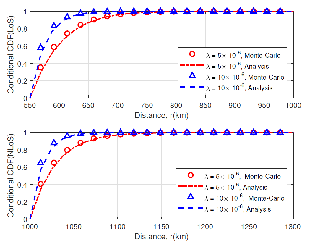
Fig. 2 plots the conditional CDFs of distance to the serving LoS and NLoS satellites for various [TeX:] $$\lambda\left(\text {units} / \mathrm{km}^2\right)$$ when when [TeX:] $$\varphi=2 \pi / 3(\mathrm{rad}) \text { and } r_{\mathrm{LN}}=1,000(\mathrm{km})$$. This figure verifies that our analytical results in (20) and (21) match well with the Monte-Carlo simulation results. We can observe from Fig. 2 that the statistical distances to the serving LoS and NLoS satellites become smaller as increases.
2) Scenario 2: [TeX:] $$r_{\mathrm{M}}(\varphi)\lt r_{\mathrm{LN}}$$: When [TeX:] $$r_{\mathrm{M}}(\varphi)\lt r_{\mathrm{LN}}$$, the typical user is always located within the beam coverage of LoS satellite only.
Lemma 4: (Association probability) When [TeX:] $$r_{\mathrm{M}}(\varphi)\lt r_{\mathrm{LN}}$$, conditioned on that there exists at least one satellite in the satellite-visible region and the typical user is located within the beam coverage of the satellite, the probability to be associated with the LoS satellite is given by
and that with NLoS satellite is given by
Proof The proof of this lemma is trivial.
Lemma 5: (Statistical distance distribution) When [TeX:] $$r_{\mathrm{M}}(\varphi)\lt r_{\mathrm{LN}}$$, conditioned on that there exists at least one satellite in satellite-visible region and the typical user is located within the beam coverage of the LoS satellite, the distance distribution to the serving satellite is given by
(24)
[TeX:] $$g_{R_0}^{\mathrm{M}, \mathrm{L}}(r)=\frac{2 \lambda \pi K r e^{-\lambda \pi K\left(r^2-H^2\right)}}{1-e^{-\lambda \pi K\left(r_{\mathrm{M}}^2(\varphi)-H^2\right)}},$$where [TeX:] $$K=\left(R_e+H\right) / R_e \text { and } H \leq r \leq r_{\mathrm{M}}(\varphi).$$
Proof This lemma can be easily obtained by following the similar proof steps of Lemma 3.
B. Analysis of Coverage Probability
The coverage probability in (11) can be re-written by
(25)
[TeX:] $$\begin{aligned} P_c(\tau) \\ =\left(\mathbb{P}\left[\operatorname{SINR} \geq \tau \mid \mathrm{E}_{\mathrm{L}}, \mathrm{E}_{\mathrm{V}}, \mathrm{E}_{\mathrm{M}}\right] \mathbb{P}\left[\mathrm{E}_{\mathrm{L}} \mid \mathrm{E}_{\mathrm{V}}, \mathrm{E}_{\mathrm{M}}\right]\right. \\ \left.+\mathbb{P}\left[\operatorname{SINR} \geq \tau \mid \mathrm{E}_{\mathrm{N}}, \mathrm{E}_{\mathrm{V}}, \mathrm{E}_{\mathrm{M}}\right] \mathbb{P}\left[\mathrm{E}_{\mathrm{N}} \mid \mathrm{E}_{\mathrm{V}}, \mathrm{E}_{\mathrm{M}}\right]\right) \mathbb{P}\left[\mathrm{E}_{\mathrm{V}}, \mathrm{E}_{\mathrm{M}}\right] \\ \end{aligned}$$
(26)
[TeX:] $$=\left(P_c^{\mathrm{M}, \mathrm{L}}(\tau) A_{\mathrm{M}, \mathrm{L}}+P_c^{\mathrm{M}, \mathrm{N}}(\tau) A_{\mathrm{M}, \mathrm{N}}\right) \mathbb{P}\left[\mathrm{E}_{\mathrm{V}}, \mathrm{E}_{\mathrm{M}}\right].$$1) Scenario 1: [TeX:] $$r_{\mathrm{M}}(\varphi) \geq r_{\mathrm{LN}}$$: Let us first consider the case of [TeX:] $$r_{\mathrm{M}}(\varphi) \geq r_{\mathrm{LN}}$$. If [TeX:] $$H \leq r \leq r_{\mathrm{LN}}$$, then the typical user can be served from the LoS satellite and experiences both LoS and NLoS interferences. If [TeX:] $$r_{\mathrm{LN}}\lt r \leq r_{\mathrm{M}}(\varphi)$$, then the typical user can be served from the NLoS satellite and experiences only NLoS interferences.
When [TeX:] $$H \leq r \leq r_{\mathrm{LN}}$$, the typical user is associated with the LoS satellite and its received SINR is given by
(27)
[TeX:] $$\mathrm{SINR}=\frac{G(\varphi) P\left|h_0\right|^2 L_0 R_0^{-\alpha_{\mathrm{L}}}}{I_1},$$where
(28)
[TeX:] $$\begin{aligned} I_1= N_0 W+\sum_{\mathbf{x}_l \in \Phi_{\mathrm{M}, \mathrm{L}} \backslash \mathrm{x}_0} G(\varphi) P\left|h_l\right|^2 L_0 R_l^{-\alpha_{\mathrm{L}}} \\ +\sum_{\mathrm{x}_l \in \Phi_{\mathrm{M}, \mathrm{N}}} G(\varphi) P\left|h_l\right|^2 L_0 R_l^{-\alpha_{\mathrm{N}}} \end{aligned}$$When [TeX:] $$r_{\mathrm{LN}}\lt r \leq r_{\mathrm{M}}(\varphi),$$ the typical user can be served from the NLoS satellite and its received SINR can be expressed as
(29)
[TeX:] $$\mathrm{SINR}=\frac{G(\varphi) P\left|h_0\right|^2 L_0 R_0^{-\alpha_{\mathrm{N}}}}{I_2},$$where
(30)
[TeX:] $$I_2=N_0 W+\sum_{\mathbf{x}_l \in \Phi_{\mathrm{M}, \mathrm{N}} \backslash \mathbf{x}_0} G(\varphi) P\left|h_l\right|^2 L_0 R_l^{-\alpha_{\mathrm{N}}}.$$Note that as [TeX:] $$\varphi$$ increases, the beam power gains of the desired link and the interfering link decrease together.
The conditional Laplace transform of aggregate interference plus noise is given as the following lemma.
Lemma 6: When the distance to the serving satellite is [TeX:] $$R_0=r$$, the conditional Laplace transform of aggregate interference plus noise is given as follows:
1) When [TeX:] $$H \leq r \leq r_{\mathrm{LN}}$$,
(31)
[TeX:] $$\begin{aligned} \mathcal{L}_{I_1}(s \mid r)=e^{-s N_0 W} \times e^{-\lambda 2 \pi\left(R_e+H\right)^2\left\{\int_{\phi(r)}^{\phi_{\mathrm{LN}}} \psi_{\mathrm{L}}(\phi) \sin \phi d \phi\right\}}\\ \times e^{-\lambda 2 \pi\left(R_e+H\right)^2\left\{\int_{\phi_{\mathrm{LN}}}^{\phi\left(r_{\mathrm{M}}(\varphi)\right)} \psi_{\mathrm{N}}(\phi) \sin \phi d \phi\right\}} \end{aligned}$$2) When [TeX:] $$r_{\mathrm{LN}} \leq r \leq r_{\mathrm{M}}(\varphi)$$,
(32)
[TeX:] $$\mathcal{L}_{I_2}(s \mid r)=e^{-s N_0 W} \times e^{-\lambda 2 \pi\left(R_e+H\right)^2\left\{\int_{\phi(r)}^{\phi\left(r_{\mathrm{M}}(\varphi)\right)} \psi_{\mathrm{N}}(\phi) \sin \phi d \phi\right\}},$$where [TeX:] $$\psi_\zeta(\phi)=1-\left(\frac{m_\zeta}{s P L_0 G(\varphi) \Omega_\zeta v(\phi)^{-\alpha}+m_\zeta}\right)^{m_\zeta}$$ for [TeX:] $$\zeta \in\{\mathrm{L}, \mathrm{N}\}$$ and [TeX:] $$\phi\left(r_{\mathrm{M}}(\varphi)\right)=\arccos \left(1-\frac{\left(r_{\mathrm{M}}(\varphi)\right)^2-H^2}{2 R_e\left(R_e+H\right)}\right)$$, where [TeX:] $$v(\phi)=\sqrt{R_e^2+\left(R_e+H\right)^2-2 R_e\left(R_e+H\right) \cos \phi}.$$
Proof The proof of this lemma is given in Appendix III.
Theorem 1: When the typical user is associated with the nearest satellite among the beam coverage satellites, the coverage probability is given by
(33)
[TeX:] $$\begin{aligned} P_c(\tau)= \left(1-e^{-\lambda \pi K\left(r_{\mathrm{M}}^2(\varphi)-H^2\right)}\right) \\ \times\left(P_c^{\mathrm{M}, \mathrm{L}}(\tau) A_{\mathrm{M}, \mathrm{L}}+P_c^{\mathrm{M}, \mathrm{N}}(\tau) A_{\mathrm{M}, \mathrm{N}}\right), \end{aligned}$$where [TeX:] $$K=\left(R_e+H\right) / R_e$$ and
(34)
[TeX:] $$P_c^{\mathrm{M}, \mathrm{L}}(\tau)=\left.\int_H^{r_{\mathrm{LN}}} \sum_{k=0}^{m_{\mathrm{L}}-1} \frac{(-s)^k}{k !} \frac{d^k}{d s^k} \mathcal{L}_{I_1}(s \mid r)\right|_{s=s_{\mathrm{L}}} f_{R_0}^{\mathrm{M}, \mathrm{L}}(r) d r,$$
(35)
[TeX:] $$P_c^{\mathrm{M}, \mathrm{N}}(\tau)=\left.\int_{r_{\mathrm{LN}}}^{r_{\mathrm{M}}(\varphi)} \sum_{k=0}^{m_{\mathrm{N}}-1} \frac{(-s)^k}{k !} \frac{d^k}{d s^k} \mathcal{L}_{I_2}(s \mid r)\right|_{s=s_{\mathrm{N}}} f_{R_0}^{\mathrm{M}, \mathrm{N}}(r) d r,$$where [TeX:] $$s_\zeta=m_\zeta \tau r^{\alpha_\zeta}\left(G(\varphi) P L_0 \Omega_\zeta\right)^{-1} \text { for } \zeta \in\{\mathrm{L}, \mathrm{N}\}.$$
Proof The proof of this theorem is given in Appendix IV.
Note that as [TeX:] $$\varphi$$ increases, the first product term in (33) increases, which implies that the beam coverage improves. However, as [TeX:] $$\varphi$$ increases, the integration range of the conditional Laplace transform of aggregated interference plus noise also increases, which implies that more larger number of satellites interferes with the user. Therefore, the optimal control of beamwidth is necessary to efficiently control the interference and the beam coverage. Unfortunately, (33) is non-convex with the very complicated form, the optimal beamwidth can be found by relying on the brute-force searching.
Corollary 1: When the typical user is associated with the nearest satellite among the beam coverage satellites, the coverage probability in the noise-limited network is given by
(36)
[TeX:] $$\begin{aligned} P_c(\tau)= \left(1-e^{-\lambda \pi K\left(r_{\mathrm{M}}^2(\varphi)-H^2\right)}\right) \\ \times\left(P_c^{\mathrm{M}, \mathrm{L}}(\tau) A_{\mathrm{M}, \mathrm{L}}+P_c^{\mathrm{M}, \mathrm{N}}(\tau) A_{\mathrm{M}, \mathrm{N}}\right), \end{aligned}$$where [TeX:] $$K=\left(R_e+H\right) / R_e$$ and
(37)
[TeX:] $$P_c^{\mathrm{M}, \mathrm{L}}(\tau)=\int_H^{r_{\mathrm{LN}}} \frac{\Gamma\left(m_{\mathrm{L}}, s_{\mathrm{L}} N_0 W\right)}{\Gamma\left(m_{\mathrm{L}}\right)} f_{R_0}^{\mathrm{M}, \mathrm{L}}(r) d r,$$
(38)
[TeX:] $$P_c^{\mathrm{M}, \mathrm{N}}(\tau)=\int_{r_{\mathrm{LN}}}^{r_{\mathrm{M}}(\varphi)} \frac{\Gamma\left(m_{\mathrm{N}}, s_{\mathrm{N}} N_0 W\right)}{\Gamma\left(m_{\mathrm{N}}\right)} f_{R_0}^{\mathrm{M}, \mathrm{N}}(r) d r,$$where [TeX:] $$s_\zeta=m_\zeta \tau r^{\alpha_\zeta}\left(G(\varphi) P L_0 \Omega_\zeta\right)^{-1} \text { for } \zeta \in\{\mathrm{L}, \mathrm{N}\}.$$
Proof The proof of this corollary can be easily derived by following the proof step of Theorem 1.
Theorem 2: When the typical user is associated with the nearest satellite among the beam coverage satellites, the coverage probability is approximated as follows:
(39)
[TeX:] $$\begin{aligned} P_c(\tau) \approx \left(1-e^{-\lambda \pi K\left(r_{\mathrm{M}}^2(\varphi)-H^2\right)}\right) \\ \times\left(\hat{P}_c^{\mathrm{M}, \mathrm{L}}(\tau) A_{\mathrm{M}, \mathrm{L}}+\hat{P}_c^{\mathrm{M}, \mathrm{N}}(\tau) A_{\mathrm{M}, \mathrm{N}}\right), \end{aligned}$$where
(40)
[TeX:] $$\begin{aligned} \hat{P}_c^{\mathrm{M}, \mathrm{L}}(\tau)= \\ \left.\int_H^{r_{\mathrm{LN}}} \sum_{n=1}^{m_{\mathrm{L}}}(-1)^{n+1}\left(\begin{array}{c} m_{\mathrm{L}} \\ n \end{array}\right) \mathcal{L}_{I_1}(s \mid r)\right|_{s=n q_{\mathrm{L}}} f_{R_0}^{\mathrm{M}, \mathrm{L}}(r) d r, \end{aligned}$$
(41)
[TeX:] $$\begin{aligned} \hat{P}_c^{\mathrm{M}, \mathrm{N}}(\tau)= \\ \left.\int_{r_{\mathrm{LN}}}^{r_{\mathrm{M}(\varphi)}} \sum_{n=1}^{m_{\mathrm{N}}}(-1)^{n+1}\left(\begin{array}{c} m_{\mathrm{N}} \\ n \end{array}\right) \mathcal{L}_{I_2}(s \mid r)\right|_{s=n q_{\mathrm{N}}} f_{R_0}^{\mathrm{M}, \mathrm{N}}(r) d r, \end{aligned}$$where [TeX:] $$q_\zeta=\eta_\zeta \kappa_\zeta(r) \text { for } \zeta \in\{\mathrm{L}, \mathrm{N}\}$$, where [TeX:] $$\eta_\zeta=m_\zeta\left(m_{\zeta} !\right)^{-1 / m_\zeta} \text { and } \kappa_\zeta(r)=\tau r^{\alpha_\zeta}\left(G(\varphi) P L_0 \Omega_\zeta\right)^{-1}.$$
Proof The proof of this theorem is given in Appendix V.
2) Scenario 2: [TeX:] $$r_{\mathrm{M}}(\varphi)\lt r_{\mathrm{LN}}$$: For the case of [TeX:] $$r_{\mathrm{M}}(\varphi)\lt r_{\mathrm{LN}}$$, the typical user can be served from the satellite only when [TeX:] $$H \leq r \leq r_M(\varphi)$$ holds. When [TeX:] $$H \leq r \leq r_M(\varphi)$$, the typical user can be served from the LoS satellite and its received SINR can be expressed as
(42)
[TeX:] $$\mathrm{SINR}=\frac{G(\varphi) P\left|h_0\right|^2 L_0 R_0^{-\alpha_{\mathrm{L}}}}{I_3},$$where
(43)
[TeX:] $$I_3=N_0 W+\sum_{\mathbf{x}_l \in \Phi_{\mathrm{M}, \mathrm{L}} \backslash \mathbf{x}_0} G(\varphi) P\left|h_l\right|^2 L_0 R_l^{-\alpha_{\mathrm{L}}}.$$Note that the typical user experiences the interferences from the LoS satellites only.
Lemma 7: When the distance to serving satellite [TeX:] $$R_0=r$$ and [TeX:] $$r_{\mathrm{M}}(\varphi)\lt r_{\mathrm{LN}}$$ holds, the conditional Laplace transform of aggregate interference is given as follows:
(44)
[TeX:] $$\mathcal{L}_{I_3}(s \mid r)=e^{-s N_0 W} e^{-\lambda 2 \pi\left(R_e+H\right)^2\left\{\int_{\phi(r)}^{\phi\left(r_{\mathrm{M}}(\varphi)\right)} \psi_{\mathrm{L}}(\phi) \sin \phi d \phi\right\}},$$where [TeX:] $$\psi_{\mathrm{L}}(\phi)=1-\left(\frac{m_{\mathrm{L}}}{s P L_0 G(\varphi) \Omega_{\mathrm{L}} v(\phi)^{-\alpha_\mathrm{L}}+m_{\mathrm{L}}}\right)^{m_{\mathrm{L}}}$$ and [TeX:] $$\phi\left(r_{\mathrm{M}}(\varphi)\right)=\arccos \left(1-\frac{\left(r_{\mathrm{M}}(\varphi)\right)^2-H^2}{2 R_e\left(R_e+H\right)}\right),$$ where [TeX:] $$v(\phi)=\sqrt{R_e^2+\left(R_e+H\right)^2-2 R_e\left(R_e+H\right) \cos \phi}.$$
Proof We omit the proof of this Lemma because it can be readily obtained by following the similar proof steps in Lemma 6.
Theorem 3: When the typical user is associated with the nearest satellite among the beam coverage satellites, the coverage probability is given by
(45)
[TeX:] $$P_c(\tau)=\left(1-e^{-\lambda \pi K\left(r_{\mathrm{M}}^2(\varphi)-H^2\right)}\right) P_c^{\mathrm{M}, \mathrm{L}}(\tau),$$where [TeX:] $$K=\left(R_e+H\right) / R_e$$ and
(46)
[TeX:] $$\begin{aligned} P_c^{\mathrm{M}, \mathrm{L}}(\tau)= \\ \left.\int_H^{r_\mathrm{M}(\varphi)} \sum_{k=0}^{m_{\mathrm{L}}-1} \frac{(-s)^k}{k !} \frac{d^k}{d s^k} \mathcal{L}_{I_3}(s \mid r)\right|_{s=s_{\mathrm{L}}} g_{R_0}^{\mathrm{M}, \mathrm{L}}(r) d r, \end{aligned}$$where [TeX:] $$s_{\mathrm{L}}=m_{\mathrm{L}} \tau r^{\alpha_{\mathrm{L}}}\left(G(\varphi) P L_0 \Omega_{\mathrm{L}}\right)^{-1}, g_{R_0}^{\mathrm{M}, \mathrm{L}}(r)$$ is given in (24), and [TeX:] $$\mathcal{L}_{I_3}(\cdot\mid\cdot)$$ is given as (44).
Proof We omit the proof of this theorem because it can be readily obtained by following the similar proof steps in Theorem 1.
Corollary 2: When the typical user is associated with the nearest satellite among the beam coverage satellites, the coverage probability in the noise-limited network is given by
(47)
[TeX:] $$P_c(\tau)=\left(1-e^{-\lambda \pi K\left(r_{\mathrm{M}}^2(\varphi)-H^2\right)}\right) P_c^{\mathrm{M}, \mathrm{L}}(\tau),$$where
(48)
[TeX:] $$P_c^{\mathrm{M}, \mathrm{L}}(\tau)=\int_H^{r_{\mathrm{M}}(\varphi)} \frac{\Gamma\left(m_{\mathrm{L}}, s_{\mathrm{L}} N_0 W\right)}{\Gamma\left(m_{\mathrm{L}}\right)} g_{R_0}^{\mathrm{M}, \mathrm{L}}(r) d r,$$where [TeX:] $$s_{\mathrm{L}}=m_{\mathrm{L}} \tau r^{\alpha_{\mathrm{L}}}\left(G(\varphi) P L_0 \Omega_{\mathrm{L}}\right)^{-1}.$$
Theorem 4: When the typical user is associated with the nearest satellite among the beam coverage satellites, the coverage probability is approximated as follows:
(49)
[TeX:] $$P_c(\tau) \approx\left(1-e^{-\lambda \pi K\left(r_{\mathrm{M}}^2(\varphi)-H^2\right)}\right) \hat{P}_c^{\mathrm{M}, \mathrm{L}}(\tau),$$where [TeX:] $$K=\left(R_e+H\right) / R_e$$ and
(50)
[TeX:] $$\begin{aligned} \hat{P}_c^{\mathrm{M}, \mathrm{L}}(\tau)= \\ \left.\int_H^{r_{\mathrm{M}}(\varphi)} \sum_{n=1}^{m_{\mathrm{L}}}(-1)^{n+1}\left(\begin{array}{c} m_{\mathrm{L}} \\ n \end{array}\right) \mathcal{L}_{I_3}(s \mid r)\right|_{s=n q_{\mathrm{L}}} g_{R_0}^{\mathrm{M}, \mathrm{L}}(r) d r, \end{aligned}$$where [TeX:] $$q_{\mathrm{L}}=\eta_{\mathrm{L}} \kappa_{\mathrm{L}}(r), \eta_{\mathrm{L}}=m_{\mathrm{L}}\left(m_{\mathrm{L}} !\right)^{-1 / m_{\mathrm{L}}} \text {, }\kappa_{\mathrm{L}}(r)=\tau r^{\alpha_{\mathrm{L}}}\left(G(\varphi) P L_0 \Omega_{\mathrm{L}}\right)^{-1}, \quad \text { and } \quad g_{R_0}^{\mathrm{M}, \mathrm{L}}(r)$$ is given(24).
Proof We omit the detailed proof because it can be readily obtained by following the similar steps in Theorem 2.
IV. ERGODIC RATES
In this section, we analyze the ergodic rates of the typical user. The technical tools and proof steps are similar to Section III, so we concisely put the derived analytical results.
The average rate of a typical user can be expressed as
(51)
[TeX:] $$R=\mathbb{E}\left[\ln (1+\mathrm{SINR}) \mid \mathrm{E}_{\mathrm{V}}, \mathrm{E}_{\mathrm{M}}\right] \mathbb{P}\left[\mathrm{E}_{\mathrm{V}}, \mathrm{E}_{\mathrm{M}}\right]$$
(52)
[TeX:] $$\begin{aligned} = \left(\mathbb{E}\left[\ln (1+\mathrm{SINR}) \mid \mathrm{E}_{\mathrm{L}}, \mathrm{E}_{\mathrm{V}}, \mathrm{E}_{\mathrm{M}}\right] \mathbb{P}\left[\mathrm{E}_{\mathrm{L}} \mid \mathrm{E}_{\mathrm{V}}, \mathrm{E}_{\mathrm{M}}\right]\right. \\ \left.+\mathbb{E}\left[\ln (1+\mathrm{SINR}) \mid \mathrm{E}_{\mathrm{N}}, \mathrm{E}_{\mathrm{V}}, \mathrm{E}_{\mathrm{M}}\right] \mathbb{P}\left[\mathrm{E}_{\mathrm{N}} \mid \mathrm{E}_{\mathrm{V}}, \mathrm{E}_{\mathrm{M}}\right]\right) \mathbb{P}\left[\mathrm{E}_{\mathrm{V}}, \mathrm{E}_{\mathrm{M}}\right] \end{aligned}$$
(53)
[TeX:] $$=\left(R_{\mathrm{M}, \mathrm{L}} A_{\mathrm{M}, \mathrm{L}}+R_{\mathrm{M}, \mathrm{N}} A_{\mathrm{M}, \mathrm{N}}\right) \mathbb{P}\left[\mathrm{E}_{\mathrm{V}}, \mathrm{E}_{\mathrm{M}}\right],$$where [TeX:] $$\mathbb{P}\left[\mathrm{E}_{\mathrm{V}}, \mathrm{E}_{\mathrm{M}}\right]=1-e^{-\lambda \pi K\left(r_{\mathrm{M}}^2(\varphi)-H^2\right)}$$ and [TeX:] $$K=\left(R_e+H\right) / R_e.$$
A. Scenario 1: [TeX:] $$r_{\mathrm{M}}(\varphi) \geq r_{\mathrm{LN}}$$
Theorem 5: When the typical user is associated with the nearest satellite among the beam coverage satellites, the ergodic rate is given by
(54)
[TeX:] $$R=\left(1-e^{-\lambda \pi K\left(r_{\mathrm{M}}^2(\varphi)-H^2\right)}\right)\left(R_{\mathrm{M}, \mathrm{L}} A_{\mathrm{M}, \mathrm{L}}+R_{\mathrm{M}, \mathrm{N}} A_{\mathrm{M}, \mathrm{N}}\right),$$where [TeX:] $$A_{\mathrm{M}, \mathrm{L}}$$ and [TeX:] $$A_{\mathrm{M}, \mathrm{N}}$$ are given in Lemma 2 and
(55)
[TeX:] $$\begin{aligned} R_{\mathrm{M}, \mathrm{L}}= \\ \left.\int_0^{\infty} \int_H^{r_{\mathrm{LN}}} \sum_{k=0}^{m_{\mathrm{L}}-1} \frac{(-s)^k}{k !} \frac{d^k}{d s^k} \mathcal{L}_{I_1}(s \mid r)\right|_{s=s_{\mathrm{L}}(r, t)} f_{R_0}^{\mathrm{M}, \mathrm{L}}(r) d r d t, \end{aligned}$$
(56)
[TeX:] $$\begin{aligned} R_{\mathrm{M}, \mathrm{N}}= \\ \left.\int_0^{\infty} \int_{r_{\mathrm{LN}}}^{r_{\mathrm{M}}(\varphi)} \sum_{k=0}^{m_{\mathrm{N}}-1} \frac{(-s)^k}{k !} \frac{d^k}{d s^k} \mathcal{L}_{I_2}(s \mid r)\right|_{s=s_{\mathrm{N}}(r, t)} f_{R_0}^{\mathrm{M}, \mathrm{N}}(r) d r d t, \end{aligned}$$Proof The proof of this theorem is placed in Appendix VI.
In the noise-limited networks, the exact expression of ergodic rates can be written as the following corollary.
Corollary 3: When the typical user is associated with the nearest satellite among the beam coverage satellites, the ergodic rate in the noise-limited network is given by
(57)
[TeX:] $$R=\left(1-e^{-\lambda \pi K\left(r_{\mathrm{M}}^2(\varphi)-H^2\right)}\right)\left(R_{\mathrm{M}, \mathrm{L}} A_{\mathrm{M}, \mathrm{L}}+R_{\mathrm{M}, \mathrm{N}} A_{\mathrm{M}, \mathrm{N}}\right),$$where
(58)
[TeX:] $$R_{\mathrm{L}}=\int_0^{\infty} \int_H^{r_{\mathrm{LN}}} \frac{\Gamma\left(m_{\mathrm{L}}, w_{\mathrm{L}}(r, t)\right)}{\Gamma\left(m_{\mathrm{L}}\right)} f_{R_0}^{\mathrm{M}, \mathrm{L}}(r) d r d t,$$
(59)
[TeX:] $$R_{\mathrm{N}}=\int_0^{\infty} \int_{r_{\mathrm{LN}}}^{r_{\mathrm{M}}(\varphi)} \frac{\Gamma\left(m_{\mathrm{N}}, w_{\mathrm{N}}(r, t)\right)}{\Gamma\left(m_{\mathrm{N}}\right)} f_{R_0}^{\mathrm{M}, \mathrm{N}}(r) d r d t,$$where [TeX:] $$w_\zeta(r, t)=m_\zeta\left(e^t-1\right) r^{\alpha_\zeta} N_0 W\left(G(\varphi) P L_0 \Omega_\zeta\right)^{-1}$$ for [TeX:] $$\zeta \in\{\mathrm{L}, \mathrm{N}\}.$$
Theorem 6: When the typical user is associated with the nearest satellite among the beam coverage satellites, the ergodic rate can be approximated as
(60)
[TeX:] $$R \approx\left(1-e^{-\lambda \pi K\left(r_{\mathrm{M}}^2(\varphi)-H^2\right)}\right)\left(\hat{R}_{\mathrm{M}, \mathrm{L}} A_{\mathrm{M}, \mathrm{L}}+\hat{R}_{\mathrm{M}, \mathrm{N}} A_{\mathrm{M}, \mathrm{N}}\right),$$where
(61)
[TeX:] $$\begin{aligned} \hat{R}_{\mathrm{M}, \mathrm{L}}= \int_0^{\infty} \int_H^{r_{\mathrm{LN}}} \sum_{n=1}^{m_{\mathrm{L}}}(-1)^{n+1}\left(\begin{array}{c} m_{\mathrm{L}} \\ n \end{array}\right) \\ \times\left.\mathcal{L}_{I_1}(s \mid r)\right|_{s=n \eta_{\mathrm{L}} \kappa_{\mathrm{L}}(r, t)} f_{R_0}^{\mathrm{M}, \mathrm{L}}(r) d r d t, \end{aligned}$$
(62)
[TeX:] $$\begin{aligned} \hat{R}_{\mathrm{M}, \mathrm{N}} =\int_0^{\infty} \int_{r_{\mathrm{LN}}}^{r_{\mathrm{M}}(\varphi)} \sum_{n=1}^{m_{\mathrm{N}}}(-1)^{n+1}\left(\begin{array}{c} m_{\mathrm{N}} \\ n \end{array}\right) \\ \times\left.\mathcal{L}_{I_2}(s \mid r)\right|_{s=n \eta_{\mathrm{N}} \kappa_{\mathrm{N}}(r, t)} f_{R_0}^{\mathrm{M}, \mathrm{N}}(r) d r d t, \end{aligned}$$where [TeX:] $$\kappa_\zeta(r, t)=\left(e^t-1\right) r^{\alpha_\zeta}\left(G(\varphi) P L_0 \Omega_\zeta\right)^{-1}$$ and [TeX:] $$\eta_\zeta=m_\zeta\left(m_{\zeta} !\right)^{-1 / m_\zeta} \text { for } \zeta \in\{\mathrm{L}, \mathrm{N}\}.$$
Proof Since the proof steps are similar to those of Theorem 2, we omit the detailed proof.
B. Scenario 2: [TeX:] $$r_{\mathrm{M}}(\varphi)\lt r_{\mathrm{LN}}$$
Theorem 7: When the typical user is associated with the nearest satellite among the beam coverage satellites, the ergodic rate is given by
(63)
[TeX:] $$R=\left(1-e^{-\lambda \pi K\left(r_{\mathrm{M}}^2(\varphi)-H^2\right)}\right) R_{\mathrm{M}, \mathrm{L}},$$where
(64)
[TeX:] $$\begin{aligned} R_{\mathrm{M}, \mathrm{L}}= \\ \left.\int_0^{\infty} \int_H^{r_{\mathrm{M}}(\varphi)} \sum_{k=0}^{m_{\mathrm{L}}-1} \frac{(-s)^k}{k !} \frac{d^k}{d s^k} \mathcal{L}_{I_3}(s \mid r)\right|_{s=s_{\mathrm{L}}(r, t)} g_{R_0}^{\mathrm{M}, \mathrm{L}}(r) d r d t, \end{aligned}$$where [TeX:] $$s_{\mathrm{L}}(r, t)=m_{\mathrm{L}}\left(e^t-1\right) r^{\alpha_{\mathrm{L}}}\left(G(\varphi) P L_0 \Omega_{\mathrm{L}}\right)^{-1}, g_{R_0}^{\mathrm{M}, \mathrm{L}}(r)$$ is given in (24), and [TeX:] $$\mathcal{L}_{I_3}(\cdot)$$ is given in Lemma 7.
Theorem 8: When the typical user is associated with the nearest satellite among the beam coverage satellites, the ergodic rate is approximated as
(65)
[TeX:] $$R=\left(1-e^{-\lambda \pi K\left(r_{\mathrm{M}}^2(\varphi)-H^2\right)}\right) \hat{R}_{\mathrm{M}, \mathrm{L}},$$where
(66)
[TeX:] $$\begin{aligned} \hat{R}_{\mathrm{M}, \mathrm{L}}= \int_0^{\infty} \int_H^{r_{\mathrm{M}}(\varphi)} \sum_{n=1}^{m_{\mathrm{L}}}(-1)^{n+1}\left(\begin{array}{c} m_{\mathrm{L}} \\ n \end{array}\right) \\ \times\left.\mathcal{L}_{I_3}(s \mid r)\right|_{s=n \eta_{\mathrm{L}} \kappa_{\mathrm{L}}(r, t)} g_{R_0}^{\mathrm{M}, \mathrm{L}}(r) d r d t, \end{aligned}$$where [TeX:] $$\kappa_{\mathrm{L}}(r, t)=\left(e^t-1\right) r^{\alpha_{\mathrm{L}}}\left(G(\varphi) P L_0 \Omega_{\mathrm{L}}\right)^{-1}$$ and [TeX:] $$\eta_{\mathrm{L}}=m_{\mathrm{L}}\left(m_{\mathrm{L}} !\right)^{-1 / m_{\mathrm{L}}}, g_{R_0}^{\mathrm{M}, \mathrm{L}}(r)$$ is given in (24), and [TeX:] $$\mathcal{L}_{I_3}(\cdot)$$ is given in Lemma 7.
V. NUMERICAL RESULTS AND DISCUSSION
In this section, we provide some numerical examples to verify our analytical results in the previous Section and provide some useful design insights. We investigate how various system parameters, such as Nakagami-m fading parameters, the pathloss exponents, the altitude, the zenith angle of LoS/NLoS transmission, and the satellite density, affect on the performances and the optimal beamwidth. Unless otherwise stated, the baseline simulation environment is set as follows [17], [18], [24]: P = 40 (dBm), H = 550 (km), [TeX:] $$\lambda=5 \times 10^{-6}\left(\text {units} / \mathrm{km}^2\right), N_0=-174(\mathrm{dBm}), f_c=2(\mathrm{GHz}),$$ [TeX:] $$W=10(\mathrm{MHz}), r_{\mathrm{LN}}=1,000(\mathrm{~km}), \alpha_{\mathrm{L}}=2, \alpha_{\mathrm{N}}=2.5,$$ [TeX:] $$m_{\mathrm{L}}=3, m_{\mathrm{N}}=2, \text { and } \Omega_{\mathrm{L}}=\Omega_{\mathrm{N}}=1.$$ In this setting, the average number of satellites over the surface of Earth is nearly 3,000.
A. Effects of Channel Fading Parameters
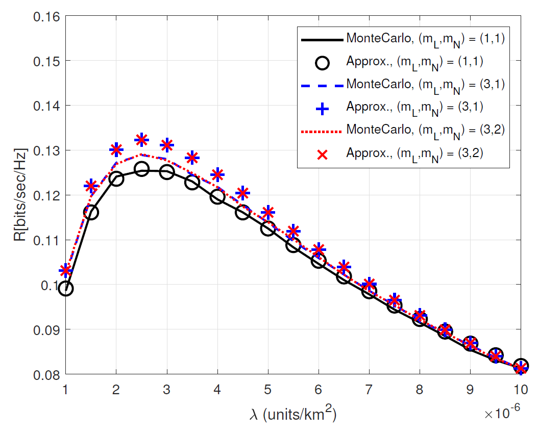
Fig. 3 and Fig. 4 compare Monte-Carlo simulated coverage probabilities and ergodic rates with their binomial approximations in (39) and (60) versus [TeX:] $$\tau(\mathrm{dB}) \text { and } \lambda \text { (units} / \mathrm{km}^2 \text {) }$$ for various [TeX:] $$m_{\mathrm{L}} \text { and } m_{\mathrm{N}}$$, respectively. These figures verify that our analytical results are quite well matched to Monte- Carlo simulation results. The gaps between the Monte-Carlo simulation and its analytical approximation become smaller as [TeX:] $$m_{\mathrm{L}} \text { and } m_{\mathrm{N}}$$ have small values. Fig. 3 shows that the coverage probabilities when [TeX:] $$\left(m_{\mathrm{L}}, m_{\mathrm{N}}\right)=(3,1) \text { and }\left(m_{\mathrm{L}}, m_{\mathrm{N}}\right)=(3,2)$$ are almost the same, while they have some gaps when [TeX:] $$\left(m_{\mathrm{L}}, m_{\mathrm{N}}\right)=(3,1) \text { and }\left(m_{\mathrm{L}}, m_{\mathrm{N}}\right)=(1,1)$$. This implies that the fading parameter for LoS link dominantly affect the coverage probability compared to that for NLoS link.
Fig. 3.
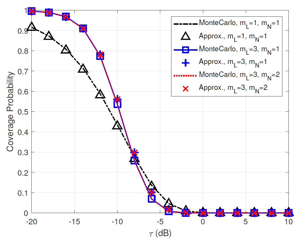
Fig. 4.
B. Effects of [TeX:] $$\lambda \text { and } r_{\mathrm{LN}}$$
Figs. 5 and 6 compare the coverage probabilities in the noise-limited and in the presence of the interferences versus [TeX:] $$\lambda\left(\text {units} / \mathrm{km}^2\right. \text {) }$$ for various [TeX:] $$r_{\mathrm{LN}}$$ (km). Fig. 5 validates that our analytical result in (36) for the noise-limited network is perfectly matched to Monte-Carlo simulation. This figure shows that the coverage probabilities increase as [TeX:] $$r_{\mathrm{LN}}$$ increases, but they are saturated for large [TeX:] $$r_{\mathrm{LN}}$$. This is because the received signal power of user increases as the probability of user to be associated with LoS transmission satellite increases. However, such gain becomes saturated as [TeX:] $$r_{\mathrm{LN}}$$ increases. Fig. 5 also shows that the coverage probabilities in the noise-limited network increase as increases. This is because the received signal power of user increases as the distance to serving satellite decreases.
Fig. 5.
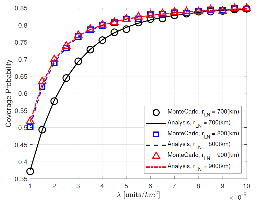
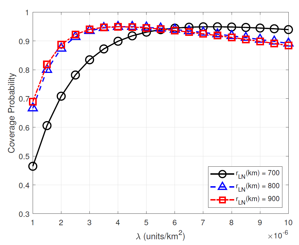
On the other hand, Fig. 6 shows that the coverage probabilities in the presence of interference increase and then decrease as increases. Obviously, as increases, the desired signal power of the typical user increases with the smaller communication distance (positive effect), but the interference also increases (negative effect). Therefore, this figure shows that the optimal control of can improve the coverage probability by effectively balancing such positive and negative effects.
Fig. 6.
C. Effects of pathloss exponents
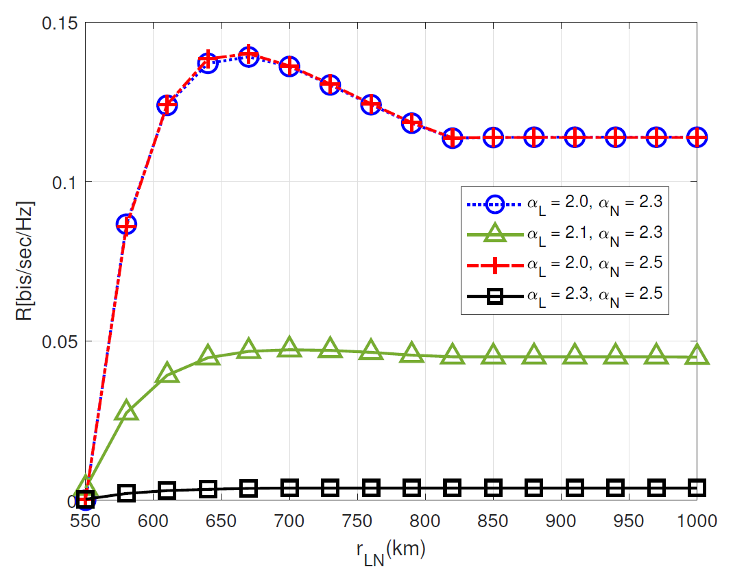
Fig. 7 compares the ergodic rates versus [TeX:] $$r_{\mathrm{LN}}$$ (km) for various [TeX:] $$\alpha_{\mathrm{L}} \text { and } \alpha_{\mathrm{N}}.$$ This figure shows that the ergodic rate increases until [TeX:] $$r_{\mathrm{LN}} \approx 670$$ (km) and then decreases and is saturated as [TeX:] $$r_{\mathrm{LN}}$$ increases. Obviously, as [TeX:] $$r_{\mathrm{LN}}$$ increases, the interference becomes more stronger but it becomes saturated. This is because more large number of satellites interferes with the user via LoS transmission rather than NLoS transmission but eventually they are saturated due to the beam coverage. Thus, Fig. 7 implies that the benefits of increasing the desired signal power with LoS communication are larger than the negative effects of increased interferences until [TeX:] $$r_{\mathrm{LN}} \approx 670$$ (km), which is vice versa for [TeX:] $$r_{\mathrm{LN}}\gt 670$$ (km). This figure also shows that the ergodic rate increases as [TeX:] $$\alpha_{\mathrm{L}}$$ decreases, while it does not vary as [TeX:] $$\alpha_{\mathrm{N}}$$ increases. This is because the maximum beam coverage distance [TeX:] $$r_{\mathrm{M}}(\varphi)$$ is smaller [TeX:] $$r_{\mathrm{LN}}$$ in our simulation setting, so the LoS transmission dominantly affects the ergodic rate and the received SINR of the user becomes higher with the smaller pathloss exponent [TeX:] $$\alpha_{\mathrm{L}}$$.
Fig. 7.
D. Effects of Altitude
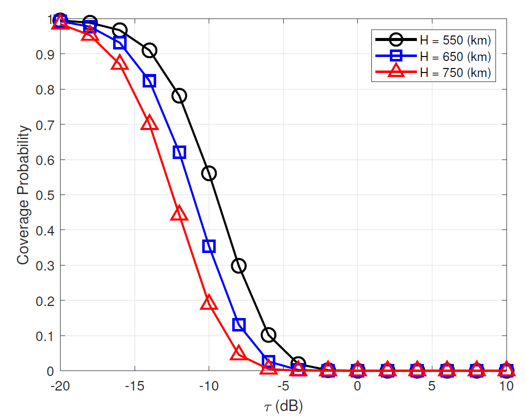
Fig. 8 depicts the coverage probabilities versus (dB) for various altitude H(km) when the average number of satellites over the entire earth orbit is fixed as 3,000 and the Earth centered zenith angle holds the same angle for all altitudes. This figure shows that the coverage probability of low altitude is higher than that of high altitude for the same average number of satellites. This implies that providing more stronger desired signal power with the small communication distance at the expense of higher interferences is more beneficial than increasing the chance of satellite visibility of user with high altitude in the satellite communication networks.
E. Effects of Beamwidth
Fig. 9 compares the coverage probabilities versus [TeX:] $$\varphi$$ (rad) for various [TeX:] $$\lambda\left(\text {units} / \mathrm{km}^2\right)$$. Fig. 9 validates that the optimal control of the beamwidth for maximizes the coverage probability. Interestingly, the optimal beamwidth decreases as increases. This is because as increases, the beamwidth coverage is sufficiently high enough even with narrow beamwidth and thus reducing the interference with the narrow beamwidth is more beneficial. On the other hand, for smaller , the beamdwidth should be more larger to guarantee the beamwidth coverage event.
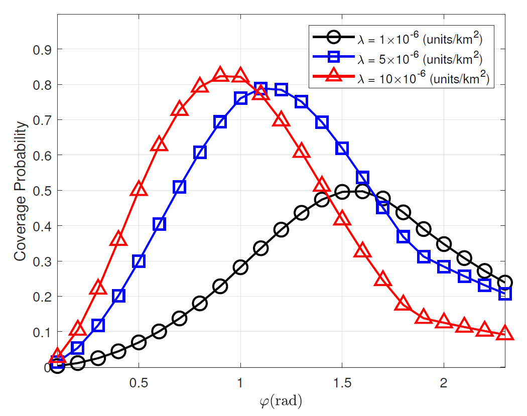
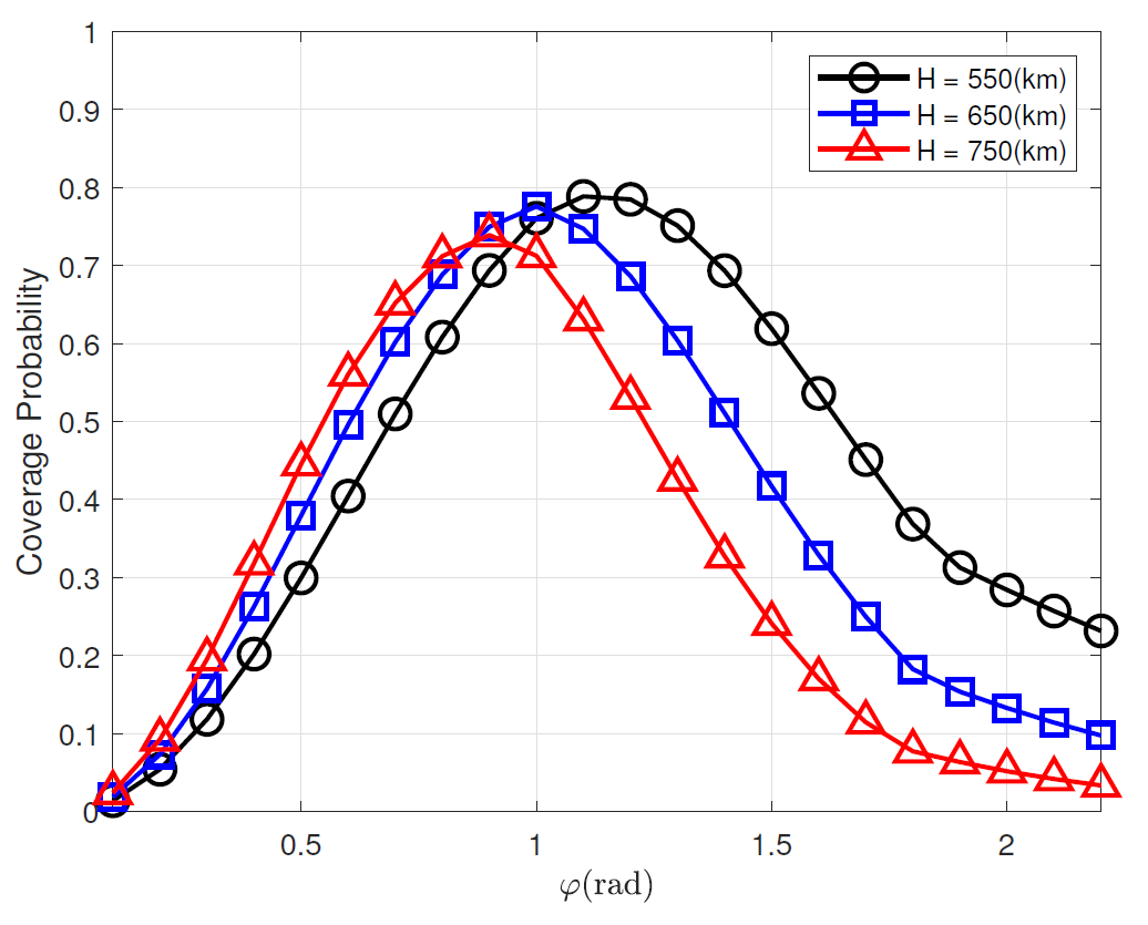
Fig. 10 compares the coverage probabilities versus [TeX:] $$\varphi$$ (rad) for various H (km) when the number of satellites are fixed as 3,000 and the zenith angle for LoS/NLoS transmission is fixed. This figure validates that the optimal beamwidth control for H maximizes the coverage probability. With the optimal beamwidth, the coverage probability of the lower altitude is more higher than that of the higher altitude. Interestingly, the optimal beamwidth for low altitude is larger than that for high altitude. This is because the beam coverage event can be guaranteed and the interference can be reduced at the higher altitude even with the narrow beamwidth.
Fig. 10.
F. Deterministic model vs PPP model
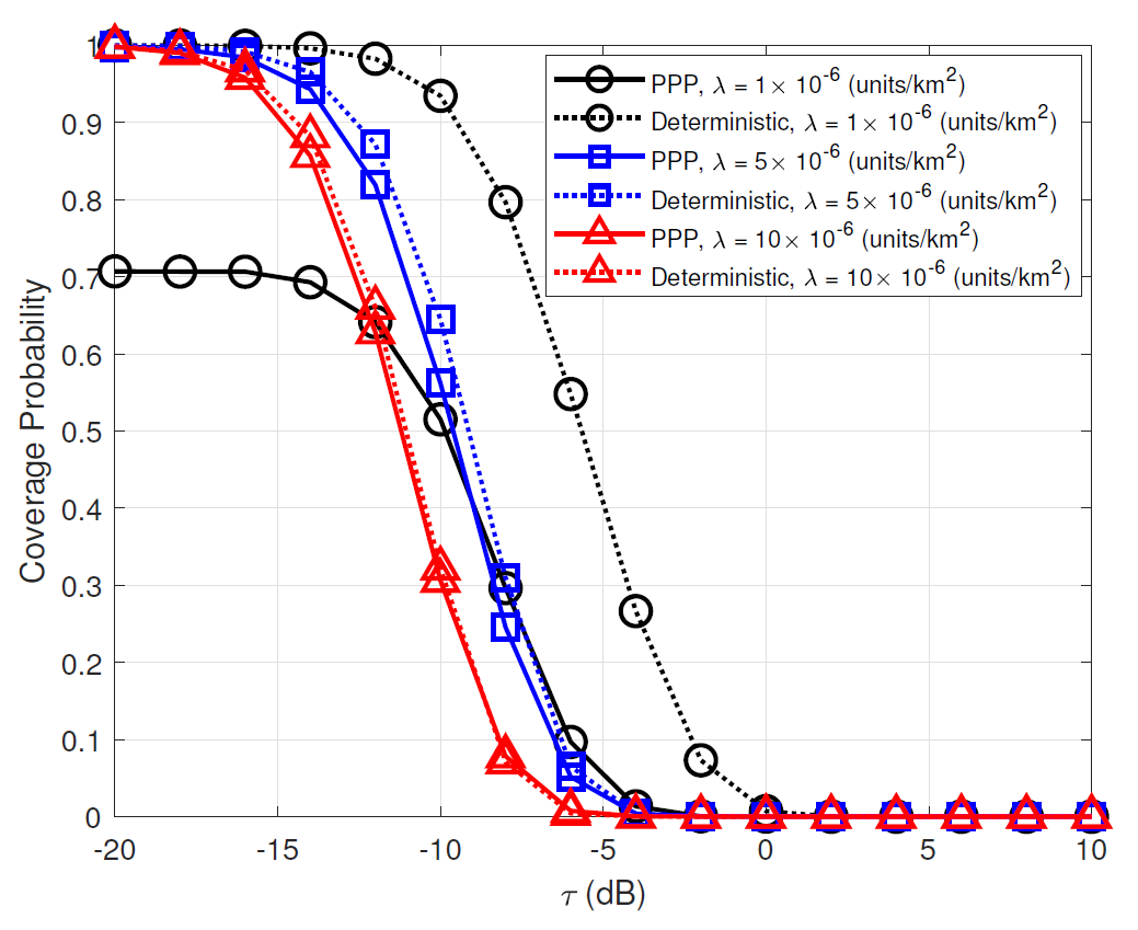
Fig. 11 compares the coverage probabilities between PPP model and deterministic model (Fibonacci lattice model) [23] versus (dB) for various [TeX:] $$\lambda\left(\text {units} / \mathrm{km}^2\right)$$. The point set of deterministic model is regularly structured with the same distance, while the point set of the PPP model is uniformly distributed. Obviously, the coverage probability of PPP model is lowerbound compared to that of deterministic model. As increases, the performance gap between two models becomes negligible. For small , there exists a large gap between two models for small . This is because the probability of beam contact in PPP model becomes more smaller than that in deterministic model for relatively small number of satellites.
VI. CONCLUSION
We have provided the analytical frameworks to analyze the downlink performance of the LEO satellite communication networks performing a directional beamforming with stochastic geometry. Based on the analytical framework, we have newly derived the exact analytical expressions for the coverage probabilities and ergodic rates over Nakagami-m fading under PPP model and their approximated formula by using binomial approximation technique. The analytical results provide us some significant design insights for how to design the optimal beamwidth to maximize the performance of the LEO satellite systems. With numerical examples, we demonstrated that the optimal control of beamwidth can maximize the performances and investigated how various system parameters, such as satellite density and altitude affect the optimal beamwidth. In uplink, the users perform the power control for their tagged satellites and thus they generate not dependent interferences. The performance analysis with not dependent interferences in uplink would be an interesting future research topic. The analysis with more sophisticated LoS/NLoS transmission model would be another interesting topic of future research.
APPENDIX A
PROOF OF LEMMA 1
Conditioned on that there exists at least one satellite in the satellite-visible region and the typical user is located within the satellite beam coverage, the CDF of the distance [TeX:] $$R_0$$ from the typical user to the nearest satellite is given by
(67)
[TeX:] $$F_{R_0}\left(r \mid \mathrm{E}_{\mathrm{V}}, \mathrm{E}_{\mathrm{M}}\right)=1-\frac{\mathbb{P}\left[R_0>r, \mathrm{E}_{\mathrm{V}}, \mathrm{E}_{\mathrm{M}}\right]}{\mathbb{P}\left[\mathrm{E}_{\mathrm{V}}, \mathrm{E}_{\mathrm{M}}\right]},$$where [TeX:] $$\mathbb{P}\left[\mathrm{E}_{\mathrm{V}}, \mathrm{E}_{\mathrm{M}}\right]=1-e^{-\lambda \pi K\left(r_{\mathrm{M}}^2(\varphi)-H^2\right)} \text { and } K=\left(R_e+\right.H) / R_e .$$ The numerator in (67) can be written by
(68)
[TeX:] $$\mathbb{P}\left[R_0>r, \mathrm{E}_{\mathrm{V}}, \mathrm{E}_{\mathrm{M}}\right]=e^{-\lambda S(r)}-e^{-\lambda S\left(r_{\mathrm{M}}(\varphi)\right)},$$where [TeX:] $$S\left(r_{\mathrm{M}}(\varphi)\right)=\pi(R e+H)\left(r_{\mathrm{M}}^2(\varphi)-H^2\right) / \mathrm{Re}$$ and [TeX:] $$S(r)=\pi(R e+H)\left(r^2-H^2\right) / R e.$$
Consequently, by plugging (68) into (67), the conditional CDF for the distance [TeX:] $$R_0$$ is given by
(69)
[TeX:] $$F_{R_0}\left(r \mid \mathrm{E}_{\mathrm{V}}, \mathrm{E}_{\mathrm{M}}\right)=\frac{1-e^{-\lambda \pi K\left(r^2-H^2\right)}}{1-e^{-\lambda \pi K\left(r_{\mathrm{M}}^2(\varphi)-H^2\right)}}.$$By taking the first derivative of [TeX:] $$F_{R_0}\left(r \mid \mathrm{E}_{\mathrm{V}}, \mathrm{E}_{\mathrm{M}}\right)$$ with respect to r, the conditional PDF of the distance [TeX:] $$R_0$$ between the typical user and the nearest satellite can be obtained as
APPENDIX B
PROOF OF LEMMA 3
When [TeX:] $$r_{\mathrm{LN}} \leq r_{\mathrm{M}}(\varphi),$$ conditioned on that there exists at least one satellite in satellite-visible region and the typical user is located within the beam coverage of LoS satellite, the conditional CDF of the distance to serving satellite can be given as
(71)
[TeX:] $$F_{R_0}^{\mathrm{L}, \mathrm{M}}(r)=\mathbb{P}\left[R_0 \leq r \mid \mathrm{E}_{\mathrm{L}}, \mathrm{E}_{\mathrm{V}}, \mathrm{E}_{\mathrm{M}}\right]$$
(72)
[TeX:] $$=\frac{\mathbb{P}\left[R_0 \leq r, \mathrm{E}_{\mathrm{L}} \mid \mathrm{E}_{\mathrm{V}}, \mathrm{E}_{\mathrm{M}}\right]}{\mathbb{P}\left[\mathrm{E}_{\mathrm{L}} \mid \mathrm{E}_{\mathrm{V}}, \mathrm{E}_{\mathrm{M}}\right]},$$where [TeX:] $$\mathbb{P}\left[\mathrm{E}_{\mathrm{L}} \mid \mathrm{E}_{\mathrm{V}}, \mathrm{E}_{\mathrm{M}}\right]=A_{\mathrm{M}, \mathrm{L}}$$ follows from Lemma 2. Then, the joint probability can be written as
(73)
[TeX:] $$\begin{aligned} \mathbb{P}\left[R_0 \leq r, \mathrm{E}_{\mathrm{L}} \mid \mathrm{E}_{\mathrm{V}}, \mathrm{E}_{\mathrm{M}}\right] \\ =1-\int_r^{r_{\mathrm{LN}}} f_{R_0}\left(r \mid \mathrm{E}_{\mathrm{V}}, \mathrm{E}_{\mathrm{M}}\right) d r \end{aligned}$$
(74)
[TeX:] $$=1-F_{R_0}\left(r_{\mathrm{LN}} \mid \mathrm{E}_{\mathrm{V}}, \mathrm{E}_{\mathrm{M}}\right)+F_{R_0}\left(r \mid \mathrm{E}_{\mathrm{V}}, \mathrm{E}_{\mathrm{M}}\right) .$$Taking the first derivative with respect to r, we can obtain
(75)
[TeX:] $$f_{R_0}^{\mathrm{M}, \mathrm{L}}(r)=\frac{d}{d r} F_{R_0}^{\mathrm{M}, \mathrm{L}}(r)=\frac{1}{A_{\mathrm{M}, \mathrm{L}}} f_{R_0}\left(r \mid \mathrm{E}_{\mathrm{V}}, \mathrm{E}_{\mathrm{M}}\right),$$where [TeX:] $$H \leq r \leq r_{\mathrm{LN}}$$. Similarly, conditioned on that there exists at least one satellite in satellite-visible region and the typical user is located within the beam coverage of NLoS satellite, the conditional distance distribution of [TeX:] $$R_0$$ can be given as
(76)
[TeX:] $$f_{R_0}^{\mathrm{M}, \mathrm{N}}(r)=\frac{1}{A_{\mathrm{M}, \mathrm{N}}} f_{R_0}\left(r \mid \mathrm{E}_{\mathrm{V}}, \mathrm{E}_{\mathrm{M}}\right),$$where [TeX:] $$r_{\mathrm{LN}} \leq r \leq r_{\mathrm{M}}(\varphi)$$ and [TeX:] $$\mathbb{P}\left[\mathrm{E}_{\mathrm{N}} \mid \mathrm{E}_{\mathrm{V}}, \mathrm{E}_{\mathrm{M}}\right]=A_{\mathrm{M}, \mathrm{N}}$$is given in Lemma 2.
APPENDIX C
PROOF OF LEMMA 6
When [TeX:] $$H \leq r \leq r_{\mathrm{LN}} \leq r_{\mathrm{M}}(\varphi),$$ conditioned on the distance to the serving satellite [TeX:] $$R_0=r,$$ the Laplace transform of the aggregate interference plus noise can be represented by
where the Laplace transform of I is given by
(80)
[TeX:] $$\begin{aligned} = \mathbb{E}_{\Phi_{\mathrm{M}, \mathrm{L}},\left|h_l\right|^2}\left[e^{-s \sum_{l>0: \mathrm{x}_l \in \Phi_{\mathrm{M}, \mathrm{L}} \backslash \mathrm{x}_0} G(\varphi) P\left|h_l\right|^2 L\left(R_l\right)}\right] \\ \times \mathbb{E}_{\Phi_{\mathrm{M}, \mathrm{N}},\left|h_l\right|^2}\left[e^{-s \sum_{l>0: \mathrm{x}_l \in \Phi_{\mathrm{M}, \mathrm{N}}} G(\varphi) P\left|h_l\right|^2 L\left(R_l\right)}\right] \end{aligned}$$
(81)
[TeX:] $$\begin{aligned} \stackrel{(a)}{=} \mathbb{E}_{\Phi_{\mathrm{M}, \mathrm{L}}}\left[\prod_{l>0: \mathbf{x}_l \in \Phi_{\mathrm{M}, \mathrm{L}} \backslash \mathbf{x}_0} \mathbb{E}_{\left|h_l\right|^2}\left[e^{-s G(\varphi) P\left|h_l\right|^2 L\left(R_l\right)}\right]\right] \\ \quad \times \mathbb{E}_{\Phi_{\mathrm{M}, \mathrm{N}}}\left[\prod_{l>0: \mathrm{x}_l \in \Phi_{\mathrm{M}, \mathrm{N}}} \mathbb{E}_{\left|h_l\right|^2}\left[e^{-s G(\varphi) P\left|h_l\right|^2 L\left(R_l\right)}\right]\right] \end{aligned}$$
(82)
[TeX:] $$\begin{aligned} \stackrel{(b)}{=} e^{-\int_{S\left(r_{\mathrm{LN}}\right) \backslash S(r)} 1-\mathbb{E}_{\left|h_l\right|^2}\left[e^{-s G(\varphi) P\left|h_l\right|^2 L\left(R_l\right)}\right] \lambda d S} \\ \quad \times e^{-\int_{S\left(r_{\mathrm{M}}(\varphi)\right) \backslash S\left(r_{\mathrm{LN}}\right)} 1-\mathbb{E}_{\left|h_l\right|^2}\left[e^{-s G(\varphi) P\left|h_l\right|^2 L\left(R_l\right)}\right] \lambda d S} . \end{aligned}$$The equality (a) comes from independence of the channel and the equality (b) holds from the probability generating functional (PGFL) of PPP. By using the moment generating function (MGF) of the Nakagami-m distribution, (82) can be written by
(83)
[TeX:] $$\begin{aligned} \mathcal{L}_I(s \mid r)= \\ e^{-\lambda 2 \pi\left(R_e+H\right)^2\left\{\int_{\phi(r)}^{\phi_{\mathrm{LN}}} 1-\left(\frac{m_{\mathrm{L}}}{s G(\varphi) P L_0 \Omega_{\mathrm{L}} v(\phi)^{-\alpha _\mathrm{L}}+m_{\mathrm{L}}}\right)^{m_{\mathrm{L}}} \sin \phi d \phi\right\}} \times e^{-\lambda 2 \pi\left(R_e+H\right)^2\left\{\int_{\phi(r)}^{\phi_{(r_\mathrm{M}(\varphi))}} 1-\left(\frac{m_{\mathrm{N}}}{s G(\varphi) P L_0 \Omega_{\mathrm{N}} v(\phi)^{-\alpha _\mathrm{N}}+m_{\mathrm{N}}}\right)^{m_{\mathrm{N}}} \sin \phi d \phi\right\}}, \end{aligned}$$where [TeX:] $$v(\phi)=\sqrt{R_e^2+\left(R_e+H\right)^2-2 R_e\left(R_e+H\right) \cos \phi}$$ and [TeX:] $$\phi\left(r_{\mathrm{M}}(\varphi)\right)=\arccos \left(1-\frac{\left(r_{\mathrm{M}}(\varphi)\right)^2-H^2}{2 R_e\left(R_e+H\right)}\right).$$ By plugging (83) into (78), we can obtain (31).
Similarly, when [TeX:] $$r_{\mathrm{LN}} \leq r \leq r_{\mathrm{M}}(\varphi)$$, the Laplace transform of the aggregate interference plus noise can be obtained as (32).
APPENDIX D
PROOF OF THEOREM 1
Conditioned on that the typical user is associated with the LoS satellite, the conditional coverage probability is given by
(84)
[TeX:] $$P_c^{\mathrm{M}, \mathrm{L}}(\tau)=\mathbb{P}\left[\mathrm{SINR} \geq \tau \mid \mathrm{E}_{\mathrm{L}}, \mathrm{E}_{\mathrm{V}}, \mathrm{E}_{\mathrm{M}}\right]$$
(85)
[TeX:] $$=\mathbb{P}\left[\frac{G(\varphi) P\left|h_0\right|^2 L_0 R_0^{-\alpha_{\mathrm{L}}}}{I_1} \geq \tau\right]$$
(86)
[TeX:] $$=\mathbb{P}\left[\left|h_0\right|^2 \geq\left(G(\varphi) P L_0\right)^{-1} R_0^{\alpha_{\mathrm{L}}} \tau I_1\right]$$
(87)
[TeX:] $$=\int_H^{r_{\mathrm{LN}}} \mathbb{E}_{I_1}\left[\frac{\Gamma\left(m_{\mathrm{L}}, s_{\mathrm{L}} I_1\right)}{\Gamma\left(m_{\mathrm{L}}\right)}\right] f_{R_0}^{\mathrm{M}, \mathrm{L}}(r) d r,$$where [TeX:] $$I_1$$ is given in (28), [TeX:] $$s_{\mathrm{L}}=m_{\mathrm{L}} \tau r^{\alpha_{\mathrm{L}}}\left(G(\varphi) P L_0 \Omega_{\mathrm{L}}\right)^{-1}$$, and [TeX:] $$f_{R_0}^{\mathrm{M}, \mathrm{L}}(r)$$ is given in (20).
Since [TeX:] $$\Gamma[m, m y] / \Gamma(m)=e^{-m y} \sum_{k=0}^{m-1}(m y)^k / k !$$ holds for any integer m [31], the following relationship holds:
(88)
[TeX:] $$\mathbb{E}_{I_1}\left[\frac{\Gamma\left(m_{\mathrm{L}}, s_{\mathrm{L}} I_1\right)}{\Gamma\left(m_{\mathrm{L}}\right)}\right]=\mathbb{E}_{I_1}\left[e^{-m_{\mathrm{L}} s_{\mathrm{L}} I_1} \sum_{k=0}^{m_{\mathrm{L}}-1} \frac{\left(s_{\mathrm{L}} I_1\right)^k}{k !}\right]$$
(89)
[TeX:] $$\left.\stackrel{(a)}{=} \sum_{k=0}^{m_{\mathrm{L}}-1} \frac{(-s)^k}{k !} \frac{d^k}{d s^k} \mathcal{L}_{I_1}(s \mid r)\right|_{s=s_{\mathrm{L}}},$$where [TeX:] $$\mathcal{L}_{I_1}(s \mid r)$$ is given in (31). The equality (a) comes from the relationship of [TeX:] $$\mathcal{L}_{x^k f(x)}(s)=(-1)^k d^k \mathcal{L}_f(s) / d s^k.$$
Using (89), we can write (87) as
(90)
[TeX:] $$P_c^{\mathrm{M}, \mathrm{L}}(\tau)=\left.\int_H^{r_{\mathrm{LN}}} \sum_{k=0}^{m_{\mathrm{L}}-1} \frac{(-s)^k}{k !} \frac{d^k}{d s^k} \mathcal{L}_{I_1}(s \mid r)\right|_{s=s_{\mathrm{L}}} f_{R_0}^{\mathrm{M}, \mathrm{L}}(r) d r.$$Similarly, conditioned on that the typical user is associated with the NLoS satellite, the conditional coverage probability is given by
(91)
[TeX:] $$\begin{aligned} P_c^{\mathrm{M}, \mathrm{N}}(\tau) \\ =\int_{r_{\mathrm{LN}}}^{r_{\mathrm{M}}(\varphi)} \mathbb{E}_{I_2}\left[\frac{\Gamma\left(m_{\mathrm{N}}, s_{\mathrm{N}} I_2\right)}{\Gamma\left(m_{\mathrm{N}}\right)}\right] f_{R_0}^{\mathrm{M}, \mathrm{N}}(r) d r, \end{aligned}$$
(92)
[TeX:] $$=\left.\int_{r_{\mathrm{LN}}}^{r_{\mathrm{M}}(\varphi)} \sum_{k=0}^{m_{\mathrm{N}}-1} \frac{(-s)^k}{k !} \frac{d^k}{d s^k} \mathcal{L}_{I_2}(s \mid r)\right|_{s=s_{\mathrm{N}}} f_{R_0}^{\mathrm{M}, \mathrm{N}}(r) d r,$$where [TeX:] $$I_2$$ is given in (30), [TeX:] $$s_{\mathrm{N}}=m_{\mathrm{N}} \tau r^{\alpha_{\mathrm{N}}}\left(G(\varphi) P L_0 \Omega_{\mathrm{N}}\right)^{-1}$$, [TeX:] $$f_{R_0}^{\mathrm{M}, \mathrm{N}}(r)$$ is given by (21), and [TeX:] $$\mathcal{L}_{I_2}(s \mid r)$$ is given in (32).
Consequently, by plugging (90) and (92) into (26), we can obtain (33).
APPENDIX E
PROOF OF THEOREM 2
Conditioned on that the typical user is associated with the LoS satellite, the conditional coverage probability can be approximated as
(93)
[TeX:] $$\begin{aligned} \hat{P}_c^{\mathrm{M}, \mathrm{L}}(\tau) \\ =\mathbb{P}\left[\mathrm{SINR} \geq \tau \mid \mathrm{E}_{\mathrm{L}}, \mathrm{E}_{\mathrm{V}}, \mathrm{E}_{\mathrm{M}}\right] \end{aligned}$$
(94)
[TeX:] $$=\int_U^{r_{\mathrm{LN}}} \mathbb{P}\left[\left|h_0\right|^2 \geq \kappa_{\mathrm{L}}(r) I_1\right] f_{R_0}^{\mathrm{M}, \mathrm{L}}(r) d r$$
(95)
[TeX:] $$\stackrel{(a)}{\approx} \int_H^{r_{\mathrm{LN}}} 1-\mathbb{E}\left[\left(1-e^{-\eta_{\mathrm{L}} \kappa_{\mathrm{L}}(r) I_1}\right)^{m_{\mathrm{L}}}\right] f_{R_0}^{\mathrm{M}, \mathrm{L}}(r) d r$$
(96)
[TeX:] $$=\left.\int_H^{r_{\mathrm{LN}}} \sum_{n=1}^{m_{\mathrm{L}}}(-1)^{n+1}\left(\begin{array}{c} m_{\mathrm{L}} \\ n \end{array}\right) \mathcal{L}_{I_1}(s \mid r)\right|_{s=n q_{\mathrm{L}}} f_{R_0}^{\mathrm{M}, \mathrm{L}}(r) d r$$where [TeX:] $$q_{\mathrm{L}}=\eta_{\mathrm{L}} \kappa_{\mathrm{L}}(r)$$, where [TeX:] $$\eta_{\mathrm{L}}=m_{\mathrm{L}}\left(m_{\mathrm{L}} !\right)^{-1 / m_{\mathrm{L}}}$$ and [TeX:] $$\kappa_{\mathrm{L}}(r)=\tau r^{\alpha_{\mathrm{L}}}\left(G(\varphi) P L_0 \Omega_{\mathrm{L}}\right)^{-1}.$$ The approximation (a) holds from the Binomial theorem.
Similarly, conditioned on that the typical user is associated with the NLoS satellite, the conditional coverage probability can be approximated as
(97)
[TeX:] $$\begin{aligned} \hat{P}_c^{\mathrm{M}, \mathrm{N}}(\tau) \\ =\mathbb{P}\left[\mathrm{SINR} \geq \tau \mid \mathrm{E}_{\mathrm{N}}, \mathrm{E}_{\mathrm{V}}, \mathrm{E}_{\mathrm{M}}\right] \end{aligned}$$
(98)
[TeX:] $$\left.\approx \int_{r_{\mathrm{LN}}}^{r_{\mathrm{M}}(\varphi)} \sum_{n=1}^{m_{\mathrm{N}}}(-1)^{n+1}\left(\begin{array}{c} m_{\mathrm{N}} \\ n \end{array}\right) \mathcal{L}_{I_2}(s \mid r)\right|_{s=n \eta_{\mathrm{N}} \kappa_{\mathrm{N}}(r)} f_{R_0}^{\mathrm{M}, \mathrm{N}}(r) d r,$$where [TeX:] $$q_{\mathrm{N}}=\eta_{\mathrm{N}} \kappa_{\mathrm{N}}(r),$$ where [TeX:] $$\eta_{\mathrm{N}}=m_{\mathrm{N}}\left(m_{\mathrm{N}} !\right)^{-1 / m_{\mathrm{N}}}$$ and [TeX:] $$\kappa_{\mathrm{N}}(r)=\tau r^{\alpha_{\mathrm{N}}}\left(G(\varphi) P L_0 \Omega_{\mathrm{N}}\right)^{-1}.$$ By plugging (96) and (98) into (26), we can derive the coverage probability as (39).
APPENDIX F
PROOF OF THEOREM 3
For a positive random variable X, the relationship of [TeX:] $$\mathbb{E}[X]=\int_{t>0} \mathbb{P}[X>t] d t$$ holds [32]. Since ln (1 + SINR) is a strictly positive random variable, the average rate [TeX:] $$R_{\mathrm{M}, \mathrm{L}}$$ can be written by
(99)
[TeX:] $$R_{\mathrm{M}, \mathrm{L}}=\mathbb{E}\left[\ln (1+\mathrm{SINR}) \mid \mathrm{E}_{\mathrm{L}}, \mathrm{E}_{\mathrm{V}}, \mathrm{E}_{\mathrm{M}}\right]$$
(100)
[TeX:] $$=\int_0^{\infty} \mathbb{P}\left[\mathrm{SINR}>e^t-1 \mid \mathrm{E}_{\mathrm{L}}, \mathrm{E}_{\mathrm{V}}, \mathrm{E}_{\mathrm{M}}\right] d t.$$Using the similar proof steps in Theorem 1, we can obtain
(101)
[TeX:] $$=\left.\int_H^{r_{\mathrm{LN}}} \sum_{k=0}^{m_{\mathrm{L}}-1} \frac{(-s)^k}{k !} \frac{d^k}{d s^k} \mathcal{L}_{I_1}(s \mid r)\right|_{s=s_{\mathrm{L}}(t)} f_{R_0}^{\mathrm{M}, \mathrm{L}}(r) d r,$$where [TeX:] $$s_{\mathrm{L}}(t)=m_{\mathrm{L}}\left(e^t-1\right) r^{\alpha_{\mathrm{L}}}\left(G(\varphi) P L_0 \Omega_{\mathrm{L}}\right)^{-1} .$$ By plugging (101) into (100), we can obtain [TeX:] $$R_{\mathrm{M}, \mathrm{L}}$$ as
(102)
[TeX:] $$\begin{aligned} R_{\mathrm{M}, \mathrm{L}} \\ =\left.\int_0^{\infty} \int_H^{r_{\mathrm{LN}}} \sum_{k=0}^{m_{\mathrm{L}}-1} \frac{(-s)^k}{k !} \frac{d^k}{d s^k} \mathcal{L}_{I_1}(s \mid r)\right|_{s=s_{\mathrm{L}}(t)} f_{R_0}^{\mathrm{M}, \mathrm{L}}(r) d r d t. \end{aligned}$$Similarly, we can also obtain [TeX:] $$R_{\mathrm{M}, \mathrm{N}}$$ as
(103)
[TeX:] $$\begin{aligned} R_{\mathrm{M}, \mathrm{N}}= \\ \left.\int_0^{\infty} \int_{r_{\mathrm{LN}}}^{r_{\mathrm{M}}(\varphi)} \sum_{k=0}^{m_{\mathrm{N}}-1} \frac{(-s)^k}{k !} \frac{d^k}{d s^k} \mathcal{L}_{I_2}(s \mid r)\right|_{s=s_{\mathrm{N}}(t)} f_{R_0}^{\mathrm{M}, \mathrm{N}}(r) d r d t . \end{aligned}$$By plugging (102) and (103) into (53), we can derive the ergodic rates as (54).
Biography
Seong Ho Chae

Seong Ho Chae received the B.S. degree from the School of Electronic and Electrical Engineering, Sungkyunkwan University, Suwon, South Korea, in 2010, and the M.S. and Ph.D. degrees from the School of Electrical Engineering, Korea Advanced Institute of Science and Technology (KAIST), Daejeon, South Korea, in 2012 and 2016, respectively. He was a Postdoctoral Research Fellow with KAIST, in 2016, and a Senior Researcher with the Agency for Defense Development, from 2016 to 2018, where he was involved in research and development for military communication system and frequency management software. He is currently an Assistant Professor with Tech University of Korea. His research interests include edge computing and caching, UAV communications, and satellite communication.
Biography
Hyeongyong Lim

Hyeongyong Lim received the B.S. and Ph.D. de- grees in Electronics and Computer Engineering from Hanyang University, Seoul, South Korea, in 2012 and 2018, respectively. Since 2018, he has been a Senior Researcher with the Defense Space Technol- ogy Center and the Defense Test & Evaluation Re- search Institute, Agency for Defense Development, Daejeon, South Korea. His research interests are in statistical signal processing with applications in detection and estimation theory, information theory, and communication theory.
Biography
Howon Lee

Howon Lee received the B.S., M.S., and Ph.D. degrees in Electrical and Computer Engineering from the Korea Advanced Institute of Science and Technology (KAIST), Daejeon, South Korea, in 2003, 2005, and 2009, respectively. From 2009 to 2012, he was a Senior Research Staff/Team Leader of the knowledge convergence team at the KAIST Institute for Information Technology Convergence (KI-ITC). Since 2012, he has been with the School of Electronic and Electrical Engineering and the Institute for IT Convergence (IITC) at Hankyong National University (HKNU), Anseong, South Korea. He has also experienced as a Visiting Scholar with the University of California, San Diego (UCSD), La Jolla, CA, USA, in 2018. His current research interests include B5G/6G wire- less communications, ultra-dense distributed networks, in-network computa- tions for 3D images, cross-layer radio resource management, reinforcement learning for UAV and satellite networks, unsupervised learning for wireless communication networks, and Internet of Things. He is the Recipient of the Joint Conference on Communications and Information (JCCI) 2006 Best Paper Award and of the Bronze Prize at Intel Student Paper Contest in 2006. Dr. Lee is also the Recipient of the Telecommunications Technology Association (TTA) Paper Contest Encour- agement Award in 2011, of the Best Paper Award at the Korean Institute of Communications and Information Sciences (KICS) Summer Conference in 2015, of the Best Paper Award at the KICS Fall Conference in 2015, of the Honorable Achievement Award from 5G Forum Korea in 2016, of the Best Paper Award at the KICS Summer Conference in 2017, of the Best Paper Award at the KICS Winter Conference in 2018, of the Best Paper Award at the KICS Summer Conference in 2018, of the Best Paper Award at the KICS Winter Conference in 2020, and of the Haedong Grand Prize at the KICS Summer Conference in 2022, and of the Haedong Grand Prize at the KICS Winter Conference in 2023. He received the Minister’s Commendation by the Minister of Science and ICT in 2017.
Biography
Bang Chul Jung
Bang Chul Jung received the B.S. degree in Elec- tronics Engineering from Ajou University, Suwon, South Korea, in 2002, and the M.S. and Ph.D. degrees in Electrical and Computer Engineering from the Korea Advanced Institute for Science and Technology (KAIST), Daejeon, South Korea, in 2004 and 2008, respectively. He was a Se- nior Researcher/Research Professor with the KAIST Institute for Information Technology Convergence, Daejeon, from 2009 to 2010. He is a Professor at the Department of Electronics Engineering, Chungnam National University, Daejeon. His research interests include wireless commu- nication systems, Internet-of-Things (IoT) communications, statistical signal processing, information theory, interference management, radio resource man- agement, spectrum-sharing techniques, and machine learning. Dr. Jung received the Fifth IEEE Communication Society Asia-Pacific Outstanding Young Researcher Award in 2011, the Bronze Prize in Intel Student Paper Contest in 2005, the First Prize in KAISTs Invention Idea Contest in 2008 and the Bronze Prize in Samsung Humantech Paper Contest in 2009. He was selected as a Winner of the Haedong Young Scholar Award in 2015, sponsored by the Haedong foundation and given by KICS. He has been selected as a Winner of the 29th Science and Technology Best Paper Award in 2019, sponsored by the Korean Federation of Science and Technology Societies. He served as an Associate Editor of IEEE VEHICULAR TECHNOLOGY MAGAZINE from 2020 to 2022, and is now a Senior Editor of IEEE VEHICULAR TECHNOLOGY MAGAZINE.
References
- 1 B. Evans, O. Onireti, T. Spathopoulous, and M. A. Imran, "The role of satellites in 5G," in Proc. EUSIPCO, Aug. 2015,doi:[[[10.1109/eusipco.2015.7362886]]]
- 2 G. Araniti, I. Bisio, M. De Sanctis, A. Orsino, and J. Cosmas, "Multimedia content delivery for emerging 5G-satellite network," IEEE Trans. Broadcast., vol. 62., no. 1, pp. 10-23, Mar. 2016.custom:[[[-]]]
- 3 N. U. Hassan, C. Huang, C. Yuen, A. Ahmad, and Y . Zhang, "Dense small satellite networks for modern terrestrial communication systems: Benefits, infrastructure, and technologies," IEEE Wireless Commun., vol. 27, no. 5, pp. 96-103, Oct. 2020.doi:[[[10.1109/mwc.001.1900394]]]
- 4 SpaceXNon-GeostationarySatelliteSystem, Federal Commun. Commissions, Washington, DC, USA, 2016.custom:[[[-]]]
- 5 OneWeb Non-Geostationary Satellite System, Federal Commun. Commissions, Washington, DC, USA, 2016.custom:[[[-]]]
- 6 X. Yue, et al., "Outage behaviors of NOMA-based satellite network over shadowed-Rician fading channels," vol. 69. no. 6, pp. 6818-6821, Jun. 2020.doi:[[[10.1109/tvt.2020.2988026]]]
- 7 Z. Wu, et al., "A graph-based satellite handover framework for LEO satellite communication networks," IEEE Commun. Lett., vol. 20, no. 8, pp. 1547-1550, Aug. 2016.doi:[[[10.1109/lcomm.2016.2569099]]]
- 8 Y . Wu, G. Hu, F. Jin, and J. Zu, "A satellite handover strategy based on the potential game in LEO satellite networks," IEEE Access, vol. 7, pp. 133461-133652, Sep. 2019.doi:[[[10.1109/access.2019.2941217]]]
- 9 L. Feng, Y . Liu, L. Wu, Z. Zhang, and J. Dang, "A satellite handover strategy based on MIMO technology in LEO satellite networks," IEEE Commun. Lett., vol. 24, no. 7, pp. 1505-1509, Jul. 2020.doi:[[[10.1109/lcomm.2020.2988043]]]
- 10 L. You, et al., "Massive MIMO transmission for LEO satellite communications," IEEE J. Sel. Areas Commun., vol. 38, no. 8, pp. 1851-1865, Aug. 2020doi:[[[10.1109/jsac.2020.3000803]]]
- 11 S. Liu, et al., "A dynamic beam shut off algorithm for LEO multibeam satellite constellation network," IEEE Wireless Commun. Lett., vol. 9, no. 10, pp. 1730-1733, Oct. 2020.doi:[[[10.1109/lwc.2020.3002846]]]
- 12 E. Wang, H. Li, and S. Zhang, "Load balancing based on cache resource allocation in satellite network," IEEE Access, vol. 7, pp. 56864-56879, Apr. 2019.custom:[[[-]]]
- 13 A. Ganz, Y . Gong, and B. Li, "Performance study of low Earthorbit satellite systems," IEEE Trans. Commun., vol. 42, no. 234, pp. 1866-1871, Feb. 1994.custom:[[[-]]]
- 14 M. Sellathurai, S. Vuppala, and T. Ratnarajah, "User selection for multibeam satellite channels: A stochastic geometry perspective," in Proc. ACSSC, Nov. 2016.custom:[[[-]]]
- 15 A. Talgat, M. A. Kishk, and M.-S. Alouini, "Nearest Neighbor and Contact Distance Distribution for Binomial Point Process on Spherical Surfaces," IEEE Commun. Lett., vol. 24, no. 12, pp. 2659-2663, Dec. 2020.doi:[[[10.1109/lcomm.2020.3019436]]]
- 16 A. Talgat, M. A. Kishk, and M.-S. Alouini, "Stochastic geometry-based analysis of LEO satellite communication systems,"IEEECommun.Lett., vol. 25, no. 8, pp. 2458-2462, Oct. 2020.doi:[[[10.1109/lcomm.2020.3029808]]]
- 17 D.-H. Jung, J.-G. Ryu, W.-J. Byun, and J. Choi, "Performance analysis of satellite communication system under the Shadowed-Rician fading: A stochastic geometry approach," IEEE Trans. Commun., vol. 70, no. 4, pp. 2707-2721, Apr. 2022.doi:[[[10.1109/tcomm.2022.3142290]]]
- 18 N. Okati, T. Riihonen, D. Korpi, I. Angervuori, and R. Wichman, "Downlink coverage and rate analysis of low earth orbit satellite constellations using stochastic geometry," IEEE Trans. Commun., vol. 68, no. 8, pp. 5120-5134, Aug. 2020.doi:[[[10.1109/tcomm.2020.2990993]]]
- 19 A. Al-Hourani, "An analytic approach for modeling the coverage performance of dense satellite networks," IEEE Wireless Commun. Lett., vol. 10, no. 4, pp. 897-901, Apr. 2021.doi:[[[10.1109/lwc.2021.3049179]]]
- 20 J. Park, J. Choi, and N. Lee, "A tractable approach to coverage analysis in downlink satellite networks," IEEE Trans. Wireless Commun, vol. 22, no. 2, pp. 793-807, Feb. 2023.doi:[[[10.1109/twc.2022.3198103]]]
- 21 N. Okati and T. Riihonen, "Nonhomogeneous stochastic geometry analysis of massive LEO communication constellations," IEEE Trans. Commun., vol. 70, no. 3, pp. 1848-1860, Mar. 2022.doi:[[[10.1109/tcomm.2022.3143131]]]
- 22 A. A.-Hourani, "Optimal satellite constellation altitude for maximal coverage," IEEE Wireless Commun. Lett., vol. 10, no. 7, pp. 1444-1448, Jul. 2021.doi:[[[10.1109/lwc.2021.3069751]]]
- 23 R. Wang, M. A. Kishk, and M.-S. Alouini, "Evaluating the accuracy of stochastic geometry based models for LEO satellite networks analysis," IEEE Commun. Lett., vol. 26, no. 10, pp. 2440-2444, Oct. 2022.doi:[[[10.1109/lcomm.2022.3194210]]]
- 24 M. Jonathan, "Starlink launch statistics," planet4589, Dec. 2022.custom:[[[-]]]
- 25 H. Xie-Dong, L. Ai-Jun, and Z. Bang-Ning, "Performance improvement using beam diversity technique in GEO satellite communication system over correlated Nakagami-m fading channels," in Proc. ICMMT, Apr. 2008.doi:[[[10.1109/icmmt.2008.4540308]]]
- 26 G. Noh, H. Chung, and I. Kim, "Outage analysis for terrestrial-satellite spectrum sharing,"IEEECommun.Lett., vol. 24, no. 10, pp. 2280-2284, Oct. 2020.doi:[[[10.1109/lcomm.2020.3006133]]]
- 27 M. Ding, P. Wang, D López-Pérez, G. Mao, and Z. Lin, "Performance impact of LoS and NLoS transmissions in dense cellular networks," IEEE Trans. Wireless Commun., vol. 15, no. 3, pp. 2365-2380, Mar. 2016.doi:[[[10.1109/twc.2015.2503391]]]
- 28 I. Atzeni, J. Arnau, and M. Kountouris, "Downlink cellular network analysis with LOS/NLOS propagation and elevated base stations," IEEE Trans. Wireless Commun., vol. 17, no. 1, pp. 142-156, Jan. 2018.doi:[[[10.1109/twc.2017.2763136]]]
- 29 O. Onireti, A. Imran, and M. A. Imran, "Coverage, capacity, and energy efficiency analysis in the uplink of mmWave cellular networks," IEEE Trans. Vehi. Tech., vol. 67, no. 5, pp. 3982-3997, May 2018.doi:[[[10.1109/tvt.2017.2775520]]]
- 30 B. Yang, M. Ding, G. Mao, X. Ge, "Performance analysis of dense small cell networks with generalized fading," in Proc. IEEE ICC, May 2017.doi:[[[10.1109/icc.2017.7997284]]]
- 31 S. H. Chae and W. Choi, "Caching placement in stochastic wireless caching helper networks: Channel selection diversity via caching," IEEE Trans. Wireless Commun., vol. 15, no. 10, pp. 6626-6637, Oct. 2016.doi:[[[10.1109/twc.2016.2586841]]]
- 32 S. H. Chae, J.-P. Hong, and W. Choi, "Optimal access in OFDMA multiRAT cellular networks with stochastic geometry: Can a single RAT be better?," IEEE Trans. Wireless Commun., vol. 15, no. 7, pp. 4778-4789, Jul. 2016.custom:[[[-]]]