José A. Cortés , Francisco J. Cañete and Luis Díez
Channel Estimation for OFDM-based Indoor Broadband Power Line Communication Systems
Abstract: State-of-the-art indoor broadband power line communications (PLC) systems use orthogonal frequency division multiplexing (OFDM) signals with constellations up to 10 bits/symbol, which makes channel estimation a key aspect. This paper focuses on the initial channel estimation used in the payload, which might be further adapted by means of a decision- directed strategy. This initial estimate has to be computed on a per-frame basis and can be accomplished from the preamble, the header symbol (assuming that it has been correctly decoded) or from a combination of both. This work proposes simple channel estimation techniques for this problem and derives their most appropriate parameters. They are compared with the linear minimum mean squared-error (LMMSE) estimator and others commonly used in wireless scenarios by considering both their performance and computational complexity. The factors limiting the performance of the estimators based on the preamble and the header symbols are analyzed and the implications of the differ- ences between PLC and wireless channels, such as the absence of fading, in the design of estimation techniques that require knowledge of the channel statistics are discussed. A performance analysis of the considered techniques is accomplished in a set of 171 measured indoor PLC channels. Obtained results indicate that estimators from the header perform better than those based on the preamble symbols and we provide a computationally simple estimator that gives nearly optimum performance by combining estimates from both the preamble and the header symbols.
Keywords: Broadband , channel estimation , OFDM , power line communications , preamble
I. INTRODUCTION
BROADBAND power line communications (PLC) is nowadays a mature technology which conveys information through the electrical wires using frequencies up to 100 MHz [1]. It is widely used for high data-rate inhome applications like the delivery of multimedia content and as a complement to wireless technologies to improve coverage. It has also been recently proposed as a backhaul technology for high data rate radiofrequency (RF) and visible light communications (VLC) systems [2] and for Internet of things (IoT) applications [3]. Broadband (BB)-PLC is also being increasingly used in Smart Grid applications like smart metering. In this context, narrowband (NB) PLC is the most extended solution in many countries [4], however, the reduced bandwidth used by NB-PLC, which is limited to the band below 500 kHz [5], is unable to convey the data rates required in some countries and is expanding the use of BB-PLC for this purpose [6]. This article focuses on broadband PLC for indoor applications which, for the sake of simplicity, will be hereafter referred simply to as PLC.
The highest performance PLC systems currently found in the market conform to the ITU-T G.hn [7]–[10] and IEEE P1901 [11] standards and the HomePlug AV2 industry specification [12]. While they are not interoperable, they all use a medium access control (MAC) with both contentionfree time division multiple access (TDMA) and carrier sense multiple access (CSMA) regions. Transmitted frames consist of a preamble with multiple predefined symbols followed by a header symbol and the payload. The intercarrier spacing used in the preamble symbols is larger than the one in the header and payload. The three systems employ orthogonal frequency division multiplexing (OFDM) modulation with constellations up to 1024 QAM, which makes accurate channel estimation a key aspect of the receiver.
This paper focuses on the initial channel estimation used in the payload, which has to be computed in each frame, and that could be subsequently adapted by means of a decisiondirected strategy when the payload has a large number of symbols. A channel estimate has to be obtained from the preamble symbols to decode the header symbol. This estimate can be further used as the initial one for the payload or can be substituted, or combined with the one obtained from the header symbol (assuming that it has been correctly decoded). In principle, the estimate obtained from the preamble has lower variance than the one from the header because of the noise reduction obtained by averaging the estimates from multiple symbols. On the other hand, it has larger bias because of the interpolation required to estimate the channel at the lower intercarrier spacing used in the payload symbols.
The linear minimum mean squared-error (LMMSE) estimator performs the optimum frequency interpolation and smoothing in the minimum mean squared-error (MMSE) sense among the class of linear estimators [13]. Hence, it is generally used as the benchmarking estimator in wireless scenarios. However, it requires perfect knowledge of the second order statistics of the channel and there is no accepted statistical model for the PLC channel response. Hence, sample autocorrelation matrices have to be used instead of the theoretical ones.
An important consideration when applying the LMMSE estimator to the considered problem is that the frequency response of PLC channels cannot be modeled as an ergodic process. Their response is determined by the physical structure of the considered indoor power network, the number and characteristics of the electrical devices connected to it and the position of the transmitter and receiver. Significant changes in the channel response occur only when electrical devices are connected/disconnected. Since this generally occurs at a rate much lower than the frame frequency, the channel can be assumed to be deterministic from the channel estimation perspective. The randomness in PLC channels is associated to changes in the indoor power network under consideration or to changes in the location of the transmitter/receiver within the same network. Hence, the expectations performed to obtain average magnitudes are computed over the ensemble of all possible PLC channels. This contrast to mobile wireless scenarios, where the channel is ergodic and the averaging is accomplished over the ensemble of states of the considered channel [14]. Hence, the effect of the mismatch due to the use of autocorrelation matrices estimated from measurements is much harmful in PLC, as it will persistently yield a poor estimation of the considered channel, and has to be explored.
Among the channel estimation techniques that require no knowledge of the channel statistics, the least-squares (LS) is the simplest one. It is the minimum variance unbiased estimator when the channel response is deterministic (as in the considered problem) and the noise is Gaussian. When the frequency response is oversampled, the mean squarederror (MSE) 1 of the estimator can be reduced, at the cost of introducing bias, by applying a low-pass filter to the estimate. However, when the coherence bandwidth of the channel is much lower than the intercarrier spacing, the noise reduction does not compensate for the introduced bias and the MSE increases. Furthermore, when the estimate is obtained from the preamble symbols, interpolation has to be also accomplished, which also introduces bias. The work in [16] studies the interpolation and noise terms caused by different interpolation techniques in an outdoor PLC modeled channel in the frequency band up to 25 MHz. However, the impact of the interpolation in the bit-rate of the physical layer (PHY) and the most appropriate bandwidth of the low-pass filter used to reduce the MSE of the estimation in actual indoor PLC channels in the band up to 100 MHz are yet unexplored.
1 The term MSE refers to the averaging of the estimates obtained in a given channel realization, which is assumed to be deterministic, while MMSE refers to the averaging of the MSE over the ensemble of channel realizations. The MMSE is also known as Bayesian MSE [15, Ch. 10].
Discrete Fourier transform (DFT)-based channel estimation was firstly proposed for wireless channels. It designates a family of techniques that reduce the estimation variance by exploiting the time-domain sparsity of the channel response, i.e., the fact that the channel energy is more concentrated in the impulse response than in the frequency response [17]. The most simple ones estimate the channel impulse response by computing the inverse discrete Fourier transform (IDFT) of a noisy estimate of the frequency response. Since only a subset of samples of the impulse response are significant (others correspond to delays with no associated propagation paths), an estimate of the channel response is obtained by computing the DFT of the most significant samples of the impulse response [18].
In wireless scenarios, these methods give good performance when the number of pilot carriers is much larger than the effective length of the impulse response. However, while the impulse response of wireless channels can be generally modeled using a relative low number of echoes, a much larger one is required in PLC. This is a consequence of the potentially infinite number of forward- and backward-traveling waves due to the reflections in the electrical cables caused by impedance mismatch [19, Ch. 5]. Furthermore, the power spectral density (PSD) of the signals transmitted in PLC has many notches in the passband imposed by electromagnetic compatibility (EMC) regulations, which may significantly affect the interpolation carried out by the DFT, as pilots are not uniformly spaced. The impact of both facts in the performance has to be quantified.
The channel estimation problem has been largely studied in PLC. However, many published works employ signals that do not conform to the existing standards [20], [21], deal with narrowband PLC systems [22]–[24] or outdoor broadband ones [21], [25]. Channels in both scenarios exhibit notable differences with respect to indoor ones. For instance, attenuation in both narrowband and broadband outdoor channels is mainly due to the conductors skin effect, while multipath is the major source in indoor broadband ones [26].
In this context, the contributions of this work are:
A study of the relevant features of PLC channels for the estimation problem, highlighting the differences with wireless scenarios. Particular emphasis is put in justifying the absence of fading in PLC, as it has been commonly misunderstood in some published works.
The proposal of several channel estimation techniques that can be applied to state-of-the-art PLC systems. Some of the considered methods are computationally simple ones based on the LS estimator. Others are grounded in strategies used in wireless channels, which are tailored to cope with particularities of the PLC scenario such as the numerous gaps in the PSD of the transmitted signal and the almost infinite number of echoes of the impulse response. Especial stress is put in discussing the use of methods, such as the LMMSE, that require knowledge of the channel statistics, which in PLC are yet unknown and have to be estimated from measurements.
A statistical analysis of the performance of these channel estimation techniques in a set of 171 measured PLC channels and the evaluation of their computational complexity. It is shown that estimation from the preamble symbols gives worse performance than from the header one and that nearly optimum performance can be achieved by using a computationally simple estimator that combines estimates obtained from both type of symbols.
The rest of the paper is organized as follows. Section II summarizes the features of the state-of-the-art PLC systems, highlighting the most relevant ones for the channel estimation problem. Section III reviews the main aspects of PLC channels and characterizes the measured channel responses and noise registers used in the performance analysis. Section IV gives the mathematical definition of the channel estimation methods whose performance and complexity is later assessed in Section V. Finally, Section VI recapitulates the main findings of the work.
Notation: Scalar variables are written using italic letters. Column vectors and matrices are written in boldface, the latter in capital letters. Sets are denoted using calligraphic letters, e.g., [TeX:] $$\mathcal{K}$$, and their cardinality as [TeX:] $$|\cdot|$$. The [TeX:] $$2 N \times 1$$ vector [TeX:] $$\mathbf{y}$$ resulting from stacking the [TeX:] $$N \times 1$$ vectors [TeX:] $$\mathbf{x}_1$$ and [TeX:] $$\mathbf{x}_2$$ is expressed as [TeX:] $$\mathbf{y}=\left[\mathbf{x}_1 ; \mathbf{x}_2\right]$$. Euclidean norm, conjugate and Hermitian operators are denoted as [TeX:] $$\|\cdot\|,(\cdot)^* \text { and }(\cdot)^H \text {, }$$ respectively. The expectation operator is denoted as [TeX:] $$\mathbb{E}[\cdot] \text { and } \circ$$ denotes the Hadamard product. The set of natural multiples of [TeX:] $$k$$ is denoted as [TeX:] $$k \mathbb{N} .$$ The [TeX:] $$N \times N$$ diagonal matrix obtained from the vector [TeX:] $$\mathbf{x}=\left[x_1, \cdots, x_N\right]$$ is denoted as diag ([TeX:] $$\mathbf{x}$$). [TeX:] $$N \times N$$ identity matrix is expressed as [TeX:] $$\mathbf{I}_N$$, while [TeX:] $$\mathbf{0}_{N \times M}$$ represents an [TeX:] $$N \times M$$ zero matrix. The 𝑁-samples DFT and IDFT of a vector [TeX:] $$\mathbf{x}$$ are denoted as [TeX:] $$\operatorname{DFT}_N[\mathbf{x}] \text { and } \operatorname{IDFT}_N[\mathbf{x}],$$ respectively.
II. FEATURES OF CURRENT PLC SYSTEMS
The ITU-T G.hn, the IEEE P1901 and the Homeplug AV2 define windowed OFDM-based PLC systems2 with flexible MAC including both centralized contention-free TDMA and CSMA regions. While they have differences like the type of forward error correcting (FEC) code and the multiple-input multiple-output (MIMO) capabilities (included in the ITU-T G.hn and Homeplug AV2 but not in the IEEE P1901), they are very similar from a preamble-based channel estimation perspective. This can be observed in Table I, where the most relevant parameters of their preambles and headers are given [1]. As seen, key parameters like the intercarrier spacing and the number of symbols in the preamble sections and in the header are equal in all of them. Hence, while this work employs the frame structure defined in the ITU-T G.hn, obtained conclusions are also applicable to the Homeplug AV2 system and, largely, to the IEEE P1901 (differences may exist because its maximum frequency is 50 MHz instead of 100 MHz).
2 The IEEE P1901 defines also a wavelet OFDM PHY with coexistence mechanisms with the OFDM-based one.
TABLE I
| Notation | Parameter | ITU-T G.hn | HomePlug AV2 | IEEE P1901 OFDM-PHY |
|---|---|---|---|---|
| [TeX:] $$f_S$$ | Maximum frequency (MHz) | 100 | 100 | 50 |
| [TeX:] $$N_p$$ | Nominal number of carriers of the preamble symbols | 512 | 512 | 256 |
| [TeX:] $$\Delta f_p$$ | Intercarrier spacing in the preamble (kHz) | 195.3125 | 195.3125 | 195.3125 |
| [TeX:] $$M_{S 1}$$ | Number of symbols in section 1 of the preamble | 7 | 7 | 7 |
| [TeX:] $$M_{S 2}$$ | Number of symbols in section 2 of the preamble | 2 | 2 | 2 |
| [TeX:] $$N_h$$ | Nominal number of carriers of the header and data symbols | 4096 | 4096 | 2048 |
| [TeX:] $$\Delta f_h$$ | Intercarrier spacing of the header and data symbols (kHz) | 24.414 | 24.414 | 24.414 |
| [TeX:] $$T_{G I}$$ | Guard interval of the header ([TeX:] $$\mu \mathrm{s}$$) | 10.24 | 18.32 | 18.32 |
| [TeX:] $$T_\beta$$ | Rolloff interval ([TeX:] $$\mu \mathrm{s}$$) | 5.12 | 4.96 | 4.96 |
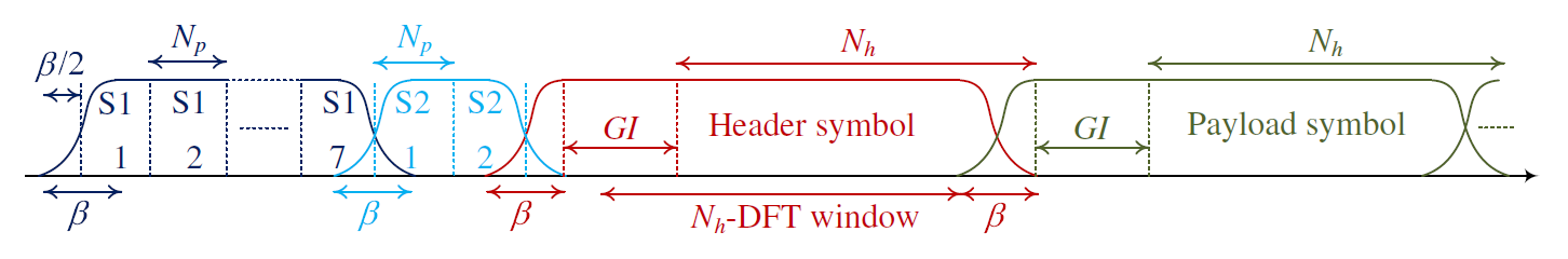
Fig. 1 depicts the discrete-time version of the frame structure defined in the ITU-T G.hn. As seen, the preamble has two sections. The first one consists of 7 repetitions of a predefined symbol, named S1, while the second is formed by the repetition of 2 symbols referred to as S2. Both the S1 and S2 symbols have no guard interval but the first and the last symbols of each series are pulse-shaped and overlapped with the preceding and following symbols, respectively. The header consists of one OFDM symbol (two in some cases) whose bits are strongly coded and modulated using QPSK. Hence, a channel estimate has to be obtained from the preamble symbols in order to decode the header symbol. Afterwards, the header can be also used to estimate the channel response.
It must be noted that the DFT performed at the receiver is computed over the [TeX:] $$N_h$$ samples labeled in Fig. 1 as [TeX:] $$\text { “N}_h-\text {DFT window"},$$ since the last [TeX:] $$\beta$$ samples of the header and payload symbols are shaped. This reduces the effective length of the (unshaped) part of the cyclic prefix to [TeX:] $$(G I-\beta)$$, causing intersymbol interference (ISI) and intercarrier interference (ICI) if the channel impulse response length exceeds this value.
The ITU-T Recommendation G.9964 defines the maximum PSD values to be used by ITU-T G.hn compliant devices, which is set to −55 dBm/kHz in the 1.1–2 MHz range, to −25 dBm/kHz between 2–30 MHz and to −55 dBm/kHz between 30–86 MHz [10]. The lower value in the high frequency band is aimed at preventing interfering other systems, as radiation becomes larger above 30 MHz. The ITU-T Rec. G.9964 also defines a set of permanently excluded subbands to avoid interfering other existing systems, such as commercial frequency modulation (FM) broadcasting services. To this end, frequencies above 86 MHz are unused in this work. While additional subbands are generally excluded by regional regulations, in this work only the set defined in the ITU-T Rec. G.9964 is employed. These notched subbands pose a problem for channel estimation, as the interpolation error increases at the edges of these subbands because of the boundary effect.
As a result of the referred notches, the set of active carriers in the preamble symbols, denoted as [TeX:] $$\mathcal{K}_p^{\mathrm{a}}$$, has cardinality [TeX:] $$\left|\mathcal{K}_p^{\mathrm{a}}\right|=N_p^{\mathrm{a}}=405$$. Similarly, the cardinality of the set of active carries in the header/data symbols is [TeX:] $$\left|\mathcal{K}_h^{\mathrm{a}}\right|=N_h^{\mathrm{a}}=3317$$. While the number of S1 symbols is 7, a reduced number is used for the channel estimation. The first ones are not useful because the automatic control gain (ACG) is still unadjusted, while the last S1 symbol and the two S2 symbols are not useful because of the ISI and ICI caused by the following/preceding symbol. Table II summarizes the values employed in this work.
TABLE II
| Notation | Parameter | Value |
|---|---|---|
| [TeX:] $$M_{S 1}^{\mathrm{v}}$$ | Number of S1 symbols valid for channel estimation | 3 |
| [TeX:] $$M_h$$ | Number of header symbols used for channel estimation | 1 |
| [TeX:] $$N_p^{\mathrm{a}}$$ | Number of active carriers in the preamble symbols | 405 |
| [TeX:] $$N_h^{\mathrm{a}}$$ | Number of active carriers in the header/data symbols | 3317 |
III. CHANNEL MODEL
Indoor power grid is formed by a set of cables of different gauge deployed from the main panel to the outlets and luminaries in a tree-like topology. Since cables are electrically long at the frequencies of the communication signal, reflections occurs due to the impedance mismatch at the cable joints, luminaries and outlets, causing a multipath propagation phenomenon [27]. Accordingly, topological models (also referred to as bottom-up) that reflect the physical structure of the electrical grid are widely employed to model PLC channels [28].
Channel response variations in PLC occur at two different time scales. The first one is due to the connection and disconnection of electrical devices, which modify the load impedance at the cable ends. These are usually referred to as long-term changes because they happen at a much lower pace (usually in the order of minutes) than the frame rate. The second type of variation is a short-term one synchronous with the mains voltage. Accordingly, the channel response can be modeled as an linear periodically time-varying (LPTV) system [29]. Fortunately, PLC channels are underspread and the slow variation approximation can be made, allowing it to be modeled as a series of time-invariant responses that repeat with the period of the mains signal [28]. Since we are interested on the initial estimation of the channel made from the preamble and the header, which lasts for about 0.52% of a 20 ms the mains period [7, Sec. 7.1.4.5.3.3.1], the channel can be assumed to be time-invariant for this purpose.
The periodic behavior of the short-term variation of PLC channels contrasts with the random nature of the small-scale fluctuations exhibited by wireless channels which, in addition, are generally much larger. However, likely the most significant difference between both channels is the non-ergodic nature of PLC ones. Since the key features of PLC channels are largely determined by the network topology and the specific path between the transmitter and the receiver, the randomness in PLC channels is mainly due to changes in the transmitter and receiver location (within the same network or placed in a different one). It must be emphasized that the ergodicity of PLC channels is a common misconception assumed in many works that assess the performance of communication systems in this scenario.
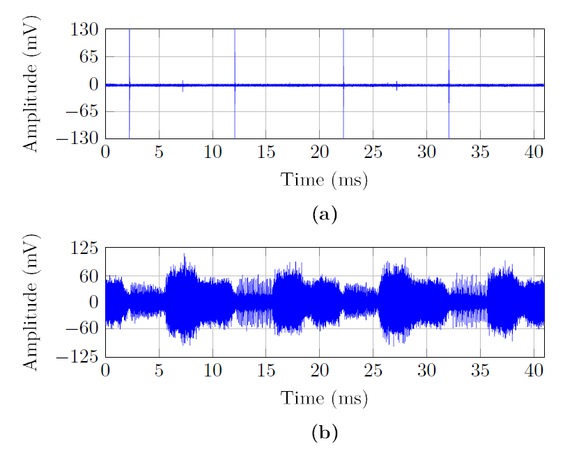
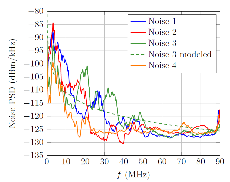
Noise in PLC is comprised of a number of terms generated by the electrical devices connected to the considered grid and others coupled to it via radiation or via conduction. According to their waveform, they can be grouped into three main categories: impulsive noise, narrowband interference and background noise [30]. Impulsive noise comprises a number of periodic components that appear at certain instants of the mains cycle, as illustrated in Fig. 2, where the waveform of two indoor noise registers measured in Spain are displayed. This determinism is a key difference with the impulsive noise typically encountered in wireless channels. The number of impulsive and narrowband terms may vary considerably among PLC networks and throughout the day, as shown in Fig. 2. Background noise can be modeled as a Gaussian colored cyclostationary process [30], [31]. However, since its variation is much slower than the preamble duration, it can be modeled as stationary for the aim of this study.
Fig. 2.
A. Channel Response
Channel responses used in this work have been obtained from a measurement campaign carried out in the indoor power networks of 22 different Spanish dwellings ranging from small flats to detached houses. The number of registered channels is [TeX:] $$Q=171$$, i.e., about 8 per dwelling. Devices plugged in the power network outlets were in their habitual location and working state. Measurements were performed employing a vectorial network analyzer using a frequency spacing of 43.125 kHz from 1–87.15 MHz. The effect of the bandpass couplers and cables was removed in the calibration process.
In the following, a statistical analysis of the coherence bandwidth and the effective length of the channel impulse response of the measured channels is given. The former measures the maximum frequency spacing over which the frequency response can be assumed to be approximately flat. Hence, it should be much larger than the intercarrier spacing. Denoting the frequency response of the considered channel by [TeX:] $$H(f),$$ its coherence bandwidth is computed as the frequency separation for which the (deterministic) autocorrelation of [TeX:] $$H(f)$$ falls down a given threshold, which in this work is set to 0.9 [32, Eq. (6)]. The effective length of the channel impulse response is defined as the length of the shortest segment of the channel impulse response that contains a given percentage of its overall energy. In this paper, the percentage is set to 99%, i.e., the energy inside this segment is 20 dB larger than the one outside.
Fig. 3.
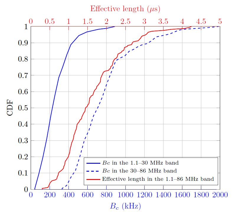
Fig. 3 depicts the empirical cumulative distribution function (CDF) of the coherence bandwidth (in blue) and the effective length (in red) of the measured channels. The coherence bandwidth is separately computed for the 1.1–30 MHz and 30–86 MHz band, while the effective length is given for the whole 1.1–86 MHz range. As seen, the amplitude response is more frequency selective in the lower band, where the median value of the coherence bandwidth is 228 kHz, whereas it is about 706 kHz in the high frequency range. The former is much larger than the intercarrier spacing of the header and payload symbols (24.41 kHz) but comparable to the 195.313 kHz spacing of the S1 symbols. This suggests that channel estimates obtained from the preamble symbols may suffer considerable interpolation error.
The analysis of the effective length of the channel impulse response is of interest because one of the estimation algorithms that will be proposed in Section IV is based on the header symbol, which might be affected by ISI and ICI if the cyclic prefix is shorter than the channel impulse response. Fig. 3 shows that all channels have effective length values lower than [TeX:] $$4.5 \mu \mathrm{s},$$ which is lower than the unshaped part of the cyclic prefix [TeX:] $$\left(T_{G I}-T_\beta=5.12 \mu \mathrm{s}\right)$$. Moreover, the effective length of about 90% of the channels is lower than half the cyclic prefix. Hence, it can be assumed that the effect of the ISI and ICI is negligible.
Fig. 4.
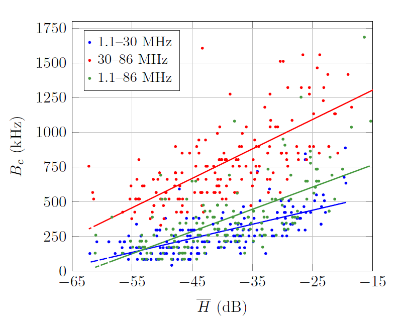
Fig. 4 shows the scatter plot of the coherence bandwidth vs the average amplitude response (averaging is performed in dB along frequencies) of the measured channels. As seen, there is a clear correlation between both magnitudes: the lower the amplitude response, the lower the coherence bandwidth. This behavior has different causes in the low and high frequency bands. In the 1–30 MHz band, attenuation is mainly due to the notches caused by the multipath propagation phenomenon. Hence, the larger (and deeper) the number of notches, the higher the attenuation and the lower the coherence bandwidth. In the 30–86 MHz band, attenuation is mainly due to the skin effect, which causes the response to exhibit a low pass behavior. Hence, the longer the link, the more pronounced the low pass behavior and the lower the coherence bandwidth. Results shown in Fig. 4 indicate that channel estimation error will be larger in highly attenuated channels both because the signal to noise ratio (SNR) will be lower and because the interpolation error will be larger.
It has been verified that the employed channels have similar features to other in-home ones reported in the literature [32], e.g., relation between delay spread and the average channel amplitude and between the delay spread and the coherence bandwidth, but a detailed comparison has been omitted for the sake of conciseness.
The performance of the estimation methods given in Section IV is assessed by means of a statistical analysis over the set of measured channels. However, for illustrative purposes, a single channel is employed to draw qualitative conclusions. Fig. 5 depicts its frequency response (in blue).
Fig. 5.
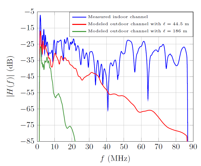
BB-PLC is being increasingly used in outdoor scenarios. Channel responses in this environment exhibit important differences with indoor ones. To highlight this end, Fig. 5 depicts the amplitude response of two low voltage (LV) outdoor PLC channels corresponding to links with lengths [TeX:] $$\ell=44.5 \mathrm{~m}$$ and [TeX:] $$\ell=186 \mathrm{~m}$$. They have been obtained using a multiconductor transmission line (MTL)-based model. As seen, the response exhibits a strong low-pass profile due to the high frequency loss caused by the skin effect and the dielectric losses, which almost eliminate the notches caused by the multipath phenomenon for frequencies above 30 MHz. In Europe, the link length of outdoor LV channels is typically in the range 150–350 m. The attenuation of the link with [TeX:] $$\ell=186 \mathrm{~m}$$ shown in Fig. 5 suggests that it is very unlikely that the frequency band above 30 MHz can be employed for communication in this scenario. Hence, the use of the channel estimation techniques proposed in this work for outdoor PLC applications requires further assessment and, in case they are deemed appropriate, would have to be adequately parameterized.
B. Noise
In this work, only background noise is considered. The reasons for disregarding impulsive and narrowband interference components are as follows. First, the background noise is always present, while the number of impulsive and narrowband terms may vary considerably, as shown in Fig. 2. Hence, considering these disturbances would make results to be highly dependent on the number of terms and the employed mitigation strategy.
Second, PLC systems generally include techniques to mitigate the influence of impulsive and narrowband components [33]. In fact, estimation techniques given in this work are also valid for proposals that take impulsive noise into account by iteratively subtracting a reconstructed version of the impulsive noise from a channel estimate obtained using off-the-self channel estimation methods [22].
Finally, the periodic behavior of the impulsive noise and narrowband interference would bias the channel estimate, hindering the relation between the frequency selectivity of the channel and the intercarrier spacing, which is one of the aims of this work.
Four representative measured noise registers are employed in this study, from which the impulsive and narrowband interference have been eliminated by exploiting their periodic features [30]. These noise registers have been selected from a set of 242 noise signals acquired in the 22 Spanish dwellings referred in Section III-A. Measurements were performed using a spectrum analyzer in the 1–210 MHz with a frequency spacing of 41.8 kHz and a resolution bandwidth of 10 kHz. The criteria employed to select the four noise registers are the noise power and the color of the PSD in the 1–86 MHz band. Fig. 6 shows the resulting power spectral densitys (PSDs), which have been selected because of their varied profile. Since PSD levels at low frequencies are much larger than at higher ones, it is commonly modeled as
with [TeX:] $$f$$ in MHz [31]. Fig. 6 displays the values of the modeled PSD corresponding to Noise 3, which will be used in Section V. The high noise levels in the low frequency band, along with the low PSD limit in the range below 2 MHz [10], make carriers in this subband useless for transmission. Consequently, they will not be used in this work.
IV. CHANNEL ESTIMATION TECHNIQUES
For coherence with the algebraic notation defined in Section I, where matrices are denoted using bold capital letters and vectors using bold lower-case, the vectors with the channel frequency and impulse response values will be denoted as [TeX:] $$\mathbf{h} \text { and } \mathbf{c} \text {, }$$, respectively. At the receiver, assuming that symbol synchronization has already been accomplished, the output of the DFT for the 𝑖th valid preamble symbol for channel estimation can then be written as
(2)
[TeX:] $$\mathbf{y}_i^p=\mathbf{X}_i^p \mathbf{h}^p+\mathbf{u}_i^p, 1 \leq i \leq M_{S 1}^{\mathrm{v}},$$where [TeX:] $$\mathbf{h}^p=\left\{h(k): k \in \mathcal{K}_p^{\mathrm{a}}\right\} \in \mathbb{C}^{N_p^{\mathrm{a}} \times 1}$$ denotes the channel frequency response in the set of frequencies corresponding to the active preamble carriers, [TeX:] $$\mathcal{K}_p^{\mathrm{a}}$$. The matrix [TeX:] $$\mathbf{X}_i^p=\operatorname{diag}\left(\mathbf{x}_i^p\right) \in \mathbb{C}^{N_p^{\mathrm{a}} \times N_p^{\mathrm{a}}}$$, with [TeX:] $$\mathbf{x}_i^p=\left\{x_i^p(k): k \in \mathcal{K}_p^{\mathrm{a}}\right\}$$, contains the complex values transmitted in the carriers of the 𝑖th preamble symbol valid for channel estimation.
The term [TeX:] $$\mathbf{u}_i^p \in \mathbb{C}^{N_p^{\mathrm{a}} \times 1}$$ denotes a Gaussian colored noise vector, which is assumed to be uncorrelated among carriers with autocorrelation matrix given by [TeX:] $$\mathbf{R}_{\mathbf{u}^p \mathbf{u}^p}=\mathbb{E}\left[\mathbf{u}^p\left(\mathbf{u}^p\right)^H\right]=\operatorname{diag}\left(\sigma_{u^p}^2\left(k_1\right), \sigma_{u^p}^2\left(k_2\right), \cdots, \sigma_{u^p}^2\left(k_{N_p^{\mathrm{a}}}\right)\right)$$ with
(3)
[TeX:] $$\sigma_{u^p}^2\left(k_i\right)=f_S \int_0^1 S_u\left(F f_S\right)\left|W_{N_p}\left(F-\frac{k_i}{N_p}\right)\right|^2 d F,$$where [TeX:] $$W_{N_p}(F)$$ is the Fourier transform of a rectangular window with [TeX:] $$N_p$$ samples, [TeX:] $$S_u(f)$$ is the noise PSD, [TeX:] $$f_S$$ is the sampling frequency and [TeX:] $$F \in[0,1)$$ is the normalized frequency.
As indicated in Table II, frames commonly have a single header symbol, which is the worst case from the channel estimation perspective, as no averaging can be made. The output of the DFT for this symbol can be expressed as
where [TeX:] $$\mathbf{h}^h=\left\{h(k): k \in \mathcal{K}_h^{\mathrm{a}}\right\} \in \mathbb{C}^{N_h^{\mathrm{a}} \times 1}$$ denotes the channel frequency response in the set of frequencies corresponding to the active header carriers, [TeX:] $$\mathcal{K}_h^{\mathrm{a}}$$. The matrix [TeX:] $$\mathbf{X}^p=\operatorname{diag}\left(\mathbf{x}^h\right) \in \mathbb{C}^{N_h^{\mathrm{a}} \times N_h^{\mathrm{a}}}$$, with [TeX:] $$\mathbf{x}^h=\left\{x^h(k): k \in \mathcal{K}_h^{\mathrm{a}}\right\},$$ contains the complex values transmitted in the carriers of the header symbol and [TeX:] $$\mathbf{u}^h \in \mathbb{C}^{N_h^{\mathrm{a}} \times 1}$$ denotes a Gaussian colored noise vector. The elements of its autocorrelation matrix, [TeX:] $$\mathbf{R}_{\mathbf{u}^h \mathbf{u}^h}=\mathbb{E}\left[\mathbf{u}^h\left(\mathbf{u}^h\right)^H\right]=\operatorname{diag}\left(\sigma_{u^h}^2\left(k_1\right), \sigma_{u^h}^2\left(k_2\right), \cdots, \sigma_{u^h}^2\left(k_{N_h^{\mathrm{a}}}\right)\right)$$ can be obtained as in (3) just by changing [TeX:] $$N_p \text { to } N_h$$.
A. LMMSE and Approximate LMMSE Estimation
The LMMSE estimator is generally used as the reference estimator for benchmarking, specially in wireless scenarios [13]. When applied to the preamble symbols, it performs interpolation and smoothing jointly, while only smoothing is accomplished when the estimate is obtained from the header symbol.
1) Estimation from the preamble symbols: Let us define [TeX:] $$\widetilde{\mathbf{y}}^p \in \mathbb{C}^{M_{S 1}^{\mathrm{v}} N_p^{\mathrm{a}} \times 1}, \quad \tilde{\mathbf{u}}^p \in \mathbb{C}^{M_{S 1}^{\mathrm{v}} N_p^{\mathrm{a}} \times 1}$$ and [TeX:] $$\widetilde{\mathbf{X}}^p \in \mathbb{C}^{M_{S 1}^{\mathrm{v}} N_p^{\mathrm{a}} \times N_p}$$ which are obtained by stacking the corresponding [TeX:] $$M_{S 1}^{\mathrm{v}}$$ vectors/matrices [TeX:] $$\mathbf{y}_i^p, \mathbf{u}_i^p \text { and } \mathbf{X}_i^p$$ in a columnwise manner, e.g., [TeX:] $$\widetilde{\mathbf{y}}^p=\left[\mathbf{y}_1^p ; \mathbf{y}_2^p ; \cdots ; \mathbf{y}_{M_{S 1}^{\mathrm{v}}}^{{p}}\right]$$ and [TeX:] $$\widetilde{\mathbf{X}}^p=\left[\operatorname{diag}\left(\mathbf{x}_1^p\right) ; \operatorname{diag}\left(\mathbf{x}_2^p\right) ; \cdots ; \operatorname{diag}\left(\mathbf{x}_{M_{S 1}^{\mathrm{v}}}^p\right)\right]$$. The output of the DFT for the [TeX:] $$M_{S 1}^{\mathrm{v}}$$ valid S1 preamble symbols can then be compactly written as
(5)
[TeX:] $$\widetilde{\mathbf{y}}^p=\widetilde{\mathbf{X}}^p \mathbf{h}^p+\widetilde{\mathbf{u}}^p$$The LMMSE estimator of the channel frequency response at the header carriers, [TeX:] $$\mathbf{h}^h \text {, }$$ can then be obtained from [15, Expr. (12.27)]. Assuming that [TeX:] $$\mathbb{E}[\mathbf{h}]=\mathbf{0}_{N_h \times 1}$$ and exploiting the particular shape of [TeX:] $$\widetilde{\mathbf{X}}^p$$ and the fact that [TeX:] $$\left|x_i^p\left(k_j\right)\right|=\left|x^p\left(k_j\right)\right|,$$ the following simplified expression is obtained after some algebra
(6)
[TeX:] $$$$ \widehat{\mathbf{h}}_{\mathrm{LMMSE-p}}^h=\mathbf{R}_{\mathbf{h}^h \mathbf{h}^p}\left(\mathbf{R}_{\mathbf{h}^p \mathbf{h}^p}+\mathbf{R}_{\mathbf{u}^p \mathbf{u}^p}\left(\left(\mathbf{X}^p\right)^H \mathbf{X}^p\right)^{-1}\right)^{-1} \\\widehat{\mathbf{\underline { h }}}_{\mathrm{LS}}^p, $$ where $\mathbf{R}_{\mathbf{h}^h \mathbf{h}^p}=\mathbb{E}\left[\mathbf{h}^h\left(\mathbf{h}^p\right)^H\right], \mathbf{R}_{\mathbf{h}^p \mathbf{h}^p}=\mathbb{E}\left[\mathbf{h}^p\left(\mathbf{h}^p\right)^H\right]$ and$$
(7)
[TeX:] $$\widehat{\mathbf{\underline { h }}}_{\mathrm{LS}}^p=\frac{1}{M_{S 1}^{\mathrm{v}}} \sum_{i=1}^{M_{S 1}^\mathrm{v}}\left(\mathbf{X}_i^p\right)^{-1} \mathbf{y}_i^p$$denotes the averaging of the LS estimates obtained from the valid preamble symbols.
Two important considerations have to be made when applying this estimator to PLC channels. First, while in wireless channels the LMMSE is obtained by averaging the error over all channel states, since PLC channels are not ergodic, the averaging has to be performed over the set of channels obtained for all possible transmitter and receiver locations. Second, the LMMSE requires the knowledge of the second order statistics of the channel response, which in PLC are yet unknown and have to be estimated from measurements. Denoting by [TeX:] $$\mathbf{h}_q^h$$ and [TeX:] $$\mathbf{h}_q^p$$ the vectors with the frequency response of the 𝑞th measured channel at the active header/payload and preamble carriers, respectively, an estimate of the channel autocorrelation matrices can be obtained as [TeX:] $$\widehat{\mathbf{R}}_{\mathbf{h}^h \mathbf{h}^p}=1 / Q \sum_{q=1}^Q \mathbf{h}_q^h\left(\mathbf{h}_q^p\right)^H$$ and [TeX:] $$\widehat{\mathbf{R}}_{\mathbf{h}^p \mathbf{h}^p}=1 / Q \sum_{q=1}^Q \mathbf{h}_q^p\left(\mathbf{h}_q^p\right)^H$$.
Fig. 7.
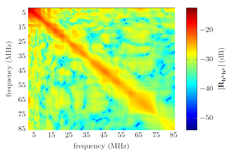
Fig. 7 depicts [TeX:] $$\left|\widehat{\mathbf{R}}_{\mathbf{h}^h \mathbf{h}^p}\right|$$ estimated from the set of 𝑄 = 171 measured channels. It reflects some of the well-known features of PLC channels. The low-pass profile of the channels manifests in the decreasing magnitude of the diagonal values as frequency increases. The width of the diagonal zone is narrower in the low frequency region than in the high frequency band, where the higher attenuation of the cables due to the skin effect reduces the depth of the notches caused by the reflected waves. This is consistent with the lower coherence bandwidth of the channel in the region below 30 MHz observed in Fig. 3.
Interestingly, the expression in (6) is formally equivalent to the one in [13], where the LMMSE estimator obtained from a single symbol is given, but substituting the LS estimate of a single symbol by the averaging of the LS estimates obtained from multiple symbols. Hence, the same strategies proposed in [13] to reduce complexity of the estimator can be employed. The first one is aimed at allowing the precomputation of the estimator matrix. Since preamble symbols are deterministic, we can write [TeX:] $$\mathbf{R}_{\mathbf{u}^p \mathbf{u}^p}\left(\left(\mathbf{X}^p\right)^H \mathbf{X}^p\right)^{-1}=\Gamma^{-1},$$ with [TeX:] $$\boldsymbol{\Gamma}=\operatorname{diag}\left(\gamma\left(k_1\right), \cdots, \gamma\left(k_{N_p^{\mathrm{a}}}\right)\right),$$ where [TeX:] $$\gamma(k)=\mathbb{E}\left[\left|x^p(k)\right|^2\right] / \sigma_{u^p}^2(k)$$ represents a sort of normalized SNR, as it does not include the effect of the channel response.
In wireless channels, where noise can be modeled as a white process and under the assumption that all pilots have the same power, the normalized SNR matrix is set to [TeX:] $$\boldsymbol{\Gamma}=\gamma_{\mathrm{obj}} \mathbf{I}_{N_p^{\mathrm{a}}}$$, where [TeX:] $$\gamma_{\text {obj }}$$ is set to a high value to avoid degrading the performance in the large SNR region [13]. This approximation is inappropriate for PLC, where the background noise is strongly colored, as shown in Fig. 6. Accordingly, we set
(8)
[TeX:] $$\mathbf{R}_{\mathbf{u}^p \mathbf{u}^p}\left(\left(\mathbf{X}^p\right)^H \mathbf{X}^p\right)^{-1}=(\lambda \boldsymbol{\Gamma})^{-1},$$where [TeX:] $$\sigma_{u^p}^2(k)$$ in [TeX:] $$\gamma(k)$$ is computed as in (3) but using the modeled PSD shown in Fig. 6 and the scaling parameter [TeX:] $$\lambda$$ is fixed to [TeX:] $$\lambda=\gamma_{\mathrm{obj}} /\left(\prod_{k \in \mathcal{K}_p^a} \gamma(k)\right)^{\left(1 / N_p^a\right)}.$$ The denominator of [TeX:] $$\lambda$$ is the geometric mean of the normalized SNR, instead of the aritmetic one, because the strongly colored nature of the noise would make the aritmetic mean to be dominated by the largest values of [TeX:] $$\gamma(k)$$, causing many carriers to have much lower normalized SNR than [TeX:] $$\gamma_{\text {obj }}$$.
The second complexity-reducing strategy consists of reducing the rank of the channel autocorrelation matrix by means of the singular value decomposition (SVD). The third one exploits the fact that the values of the channel response at frequency separations much larger than the coherence bandwidth are uncorrelated and, hence, carriers can be partitioned into subsets in which the channel estimation is performed independently. To reduce the boundary effect, these subsets can overlap, computing the correlation matrices over a larger set of carriers than the ones in which the frequency response will be estimated. The resulting estimator is referred to as approximate LMMSE (aLMMSE).
Despite these strategies, the aLMMSE estimator still has a high complexity and degraded performance due to the use of correlation matrices estimated from measurements and a fixed objective SNR value. Moreover, since in PLC each channel realization is associated to a different transmitter and receiver location, a bad estimate remains until a long-term change occurs.
2) Estimation from the header symbol: The LMMSE estimator can also operate over the LS estimate obtained from the header symbol in (4), assuming that [TeX:] $$\mathbf{X}^h$$ has been correctly decoded,
yielding
(10)
[TeX:] $$$$ \widehat{\mathbf{h}}_{\mathrm{LMMSE-h}}^h=\mathbf{R}_{\mathbf{h}^h \mathbf{h}^h}\left(\mathbf{R}_{\mathbf{h}^h \mathbf{h}^h}+\mathbf{R}_{\mathbf{u}^h \mathbf{u}^h}\left(\left(\mathbf{X}^h\right)^H \mathbf{X}^h\right)^{-1}\right)^{-1} \widehat{\underline{\mathbf{h}}}_{\mathrm{LS}}^h, $$ where $\mathbf{R}_{\mathbf{h}^h \mathbf{h}^h}=\mathbb{E}\left[\mathbf{h}^h\left(\mathbf{h}^h\right)^H\right]$$$The LMMSE-h can benefit from the same complexity reduction strategies described for the LMMSE-p estimator. However, the resulting computational cost still makes it unpractical. Hence, in this work it will be used just to upper bound the performance.
B. LS Estimation with Frequency-Domain (FD) Processing
1) Estimation from the preamble symbols: Suboptimal but computationally simpler estimators can be obtained by substituting the inherent interpolation performed in the aLMMSE by a piecewise polynomial interpolation of the average LS estimate given in (7). Two interpolation methods are assessed: linear and cubic. Since [TeX:] $$N_h / N_p=8$$, when linear interpolation is employed, the 3 values of the frequency response in the header/payload carriers located between the active preamble carriers [TeX:] $$k_{p_i}$$ and [TeX:] $$k_{p_{i+1}}$$ are obtained as
(11)
[TeX:] $$\begin{aligned} \widehat{h}_{\mathrm{LIN}-\mathrm{p}}^h(k)= & \frac{k-8 k_{p_i}}{8 k_{p_{i+1}}-8 k_{p_i}}\left(\widehat{\underline{h}}_{\mathrm{LS}}^p\left(8 k_{p_{i+1}}\right)-\widehat {\underline{h}}_{\mathrm{LS}}^p\left(8 k_{p_i}\right)\right) \\ & +\widehat{\underline{h}}_{\mathrm{LS}}^p\left(8 k_{p_i}\right), \end{aligned}$$for [TeX:] $$8 k_{p_i}+1 \leq k \leq 8 k_{p_i}+7$$, while [TeX:] $$\widehat{h}_{\mathrm{LIN}-\mathrm{p}}^h(k)=\widehat{\underline{h}}_{\mathrm{LS}}^p\left(8 k_{p_i}\right)$$ when [TeX:] $$k \in \mathcal{K}_h^{\mathrm{a}} \cap 8 \mathbb{N}$$.
When piecewise cubic interpolation is employed, the frequency points must be uniformly spaced. Since the notches in the PSD prevent [TeX:] $$\widehat{\underline{\mathbf{h}}}_{\mathrm{LS}}^p$$ from fulling this condition. The values of [TeX:] $$\widehat{\underline{h}}_{\mathrm{LS}}^p(k)$$ in the notched carriers are first obtained by linear interpolation. Then, the values of the estimated vector [TeX:] $$\widehat{\mathbf{h}}_{\text {CUB-p }}^h$$ are obtained from the interpolated vector as indicated in [34].
2) Estimation from the header symbol: This method firstly computes the LS estimate of the channel at the frequency of the valid header carriers, as given in (9). The estimation variance is reduced by applying a sliding window filter to it. However, the multiple gaps in the PSD of the transmitted signal cause the filtering to suffer from a boundary effect that degrades the performance. This can be reduced by estimating the values of the frequency response in the notched regions using piecewise linear interpolation yielding, [TeX:] $$\widehat{h}_{\text {LS-INT}}^h(k)$$.
The final estimate [TeX:] $$\widehat{\mathbf{h}}_{\mathrm{FD}-\mathrm{h}}^h$$ is then obtained by filtering the elements in [TeX:] $$\widehat{\mathbf{h}}_{\text {LS-INT }}^h$$ with a sliding window filter of length [TeX:] $$L_{s w}$$,
(12)
[TeX:] $$\widehat{h}_{\mathrm{FD}-\mathrm{h}}^h(k)=\frac{1}{L_{s w}} \sum_{i=-\left(L_{s w}-1\right) / 2}^{\left(L_{s w}-1\right) / 2} \widehat{h}_{\mathrm{LS-INT}}^h(k+i), \quad k \in \mathcal{K}_h^{\mathrm{a}}.$$C. DFT-based Channel Estimation
The time-domain sparsity of the channel response can be exploited by estimating its impulse response, by applying the IDFT to a noisy estimate of the channel frequency response, and returning to the frequency domain by computing the DFT of the most significant samples (MSS) of the impulse response [35]. Furthermore, this DFT can be also used to perform frequency-domain interpolation when the number of pilot carriers is lower than the number of data carriers, as DFT interpolation is optimal in a noiseless scenario and with sufficient pilot density [18].
In the considered problem, DFT-based estimation can be applied to the preamble symbols. In this case, it is used just as an interpolation technique. No MSS selection is performed because it requires the number of selected samples to be much larger (twice or even more) than the effective length of the channel impulse response to avoid the error floor caused by the discarded samples [35]. As displayed in Fig. 3, the effective length of the impulse response of 50% of the channels is larger than [TeX:] $$1.5 \mu \mathrm{s}$$, which at [TeX:] $$f_S=100 \mathrm{MHz}$$ yields 150 samples. Hence, almost all the [TeX:] $$N_p$$ samples of the channel impulse response estimated from the preamble symbols have to be considered. Moreover, the distortion caused by the discarded samples is aggravated by the time-aliasing that occurs in the IDFT. This is caused by the frequency-domain undersampling that occurs because the intercarrier spacing is comparable to the coherence bandwidth in the low frequency band. Furthermore, the notches in the PSD of the transmitted signal aggravates the time-domain aliasing, which in turn causes bias. On the other hand, the averaging of the useful S1 symbols reduces the estimation variance by [TeX:] $$10 \log _{10}\left(M_{S 1}^{\mathrm{v}}\right) \mathrm{dB} .$$
DFT-based estimation can be also applied to the header symbol. In this case, no bias occur because the frequency response is oversampled but the noise reduction achieved by MSS selection depends on the effective number of samples of the impulse response.
1) Estimation from preamble symbols: This method starts with the averaging of the LS estimates of the frequency response obtained from the S1 symbols given in (7). This vector is then extended to [TeX:] $$N_p$$ elements, with zero padding of the frequencies below 2 MHz and above 86 MHz, while the ones located in notched regions of the passband are computed by linearly interpolating the values of the carriers located at the edges of the corresponding notch. The resulting vector is denoted as [TeX:] $$\widehat{\mathbf{h}}_{\text {LS-ext }}^p$$.
The estimate of the channel impulse response is obtained by computing the IDFT of [TeX:] $$\widehat{\mathbf{h}}_{\text {LS-ext }}^p$$,
(13)
[TeX:] $$\widehat{\mathbf{c}}^p=\operatorname{IDFT}_{N_p}\left[\mathbf{s}^p \circ \widehat{\mathbf{h}}_{\mathrm{LS}-\mathrm{ext}}^p\right],$$where [TeX:] $$\mathbf{S}^p \in \mathbb{R}^{N_p \times 1}$$ is a spectral shaping window with [TeX:] $$N_p^a$$ nonzero samples of which the first and last [TeX:] $$\alpha^p$$ ones are shaped using a Hanning window. This shaping prevents the sinc-type time-domain waveforms associated to the steep transitions of the frequency response that would artificially enlarge the impulse response.
An estimate of the frequency response (at all carrier frequencies) is then obtained by calculating the DFT of a zeropadded version of [TeX:] $$\widehat{\mathbf{c}}^p$$,
(14)
[TeX:] $$\widehat{\mathbf{h}}_{\mathrm{DFT}-\mathrm{p}}^h=\operatorname{DFT}_{N_h}\left[\left[\widehat{\mathbf{c}}^p ; \mathbf{0}_{\left(N_h-N_p\right) \times 1}\right]\right].$$2) Estimation from the header symbol: This method assumes that the header symbol has been correctly decoded. To this end, a coarse estimation of the channel frequency response must have been previously performed using a preamble-based estimator. The following steps are then applied.
First, the LS estimate of the channel frequency response at the frequency of the [TeX:] $$N_h^{\mathrm{a}}$$ active data carriers is obtained according to (9). This vector is then extended to [TeX:] $$N_h$$ elements, yielding [TeX:] $$\widehat{\mathbf{h}}_{\text {LS-ext }}^h$$. As in the DFT-p method, the padded elements corresponding to the frequencies below 2 MHz and above 86 MHz are set to zero, while the ones located in notched regions of the passband are computed by linear interpolation of the values located at the edges of the corresponding notch.
An estimate of the impulse response is then obtained as
(15)
[TeX:] $$\widehat{\mathbf{c}}^h=\operatorname{IDFT}_{N_h}\left[\mathbf{s}^h \circ \widehat{\mathbf{h}}_{\mathrm{LS}-\mathrm{ext}}^h\right],$$where [TeX:] $$\mathbf{s}^h \in \mathbb{R}^{N_h \times 1}$$ plays the same role as [TeX:] $$\mathbf{S}^p$$ is the DFT-p method but with [TeX:] $$N_h^a$$ non-zero samples of which the first and last [TeX:] $$\alpha^h$$ ones are shaped using a Hanning window.
Since the effective length of the impulse response is much shorter than [TeX:] $$N_h$$, the estimator variance can be reduced by the DFT of the MSS of [TeX:] $$\widehat{\mathbf{c}}^h$$ and returning to the frequency domain,
(16)
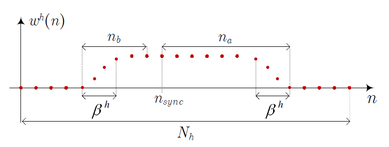
[TeX:] $$\widehat{\mathbf{h}}_{\mathrm{DFT}-\mathrm{h}}^h=\mathrm{DFT}_{N_h}\left[\mathbf{w}^h \circ \widehat{\mathbf{c}}^h\right],$$where [TeX:] $$\mathbf{w}^h \in \mathbb{R}^{N_h \times 1}$$ is a window with [TeX:] $$n_a+n_b$$ non-zero samples, [TeX:] $$n_b$$ located before the sample index given by the synchronization algorithm, [TeX:] $$n_{\text {sync }}$$ (usually located around the maximum absolute value of [TeX:] $$\widehat{\mathbf{c}}^h$$) and [TeX:] $$n_a$$ samples after it. Fig. 8 shows the waveform of [TeX:] $$\mathbf{w}^h$$, where the [TeX:] $$\beta^h \text {-samples }$$ shaped regions are generated using a Hanning window.
D. Combined Estimation from the Preamble and Header Symbols
An improved estimation can be obtained by combining the estimates obtained from the preamble and the header symbols. Let us denote these estimates by [TeX:] $$\widehat{\mathbf{h}}_{\mathrm{X}-\mathrm{p}}^h \text { and } \widehat{\mathbf{h}}_{\mathrm{Y}-\mathrm{h}}^h \text {, }$$ where X and Y refer to any of the preamble and header-based methods presented above, respectively. Denoting by [TeX:] $$\rho_k$$ the ratio of the variance of the header estimator to the variance of the preamble one in carrier 𝑘, a combined estimate can be obtained as3
3 Expression (17) is optimum when the estimation errors are zero-mean and independent.
(17)
[TeX:] $$\widehat{\mathbf{h}}_{\mathrm{COMB}}^h(k)=\frac{\rho_k \widehat{\mathbf{h}}_{\mathrm{X}-\mathrm{p}}^h(k)+\widehat{\mathbf{h}}_{\mathrm{Y}-\mathrm{h}}^h(k)}{1+\rho_k} .$$In carriers that are multiple of [TeX:] $$N_h / N_p=8$$, the averaging of the preamble symbols reduces the variance of the LS estimator by [TeX:] $$M_{S 1}^{\mathrm{v}}$$ (further reduction might be achieved when the aLMMSE is employed), while the noise reduction in the header-based estimator is achieved by means of the frequencydomain smoothing in the FD-h and by means of the MSS selection in the DFT-h. In the remaining carriers, [TeX:] $$k \notin 8 \mathbb{N},$$ the value of [TeX:] $$\rho_k$$ depends on the relative magnitude of the bias of the preamble-based estimator and of the variance of the header-based one. Hence, the optimum value of [TeX:] $$\rho_k$$ has to be determined by simulation.
V. PERFORMANCE ANALYSIS
This section compares the performance and the implementation complexity of the presented channel estimators. The parameters of the aLMMSE, FD-h and DFT-h estimators are firstly selected. Then, a statistical analysis of the performance loss due to the estimation errors in the set of measured channels is given.
A. Estimators Parameterization
For illustrative purposes, results given in this section are obtained in an example channel consisting of the frequency response shown in Fig. 5 and the noise PSD labeled as Noise 3 in Fig. 6. The PSD of the transmitted signal in the 30–86 MHz band is 30 dB lower than in the 2–30 MHz range (as in the ITU-T G.hn), but their absolute values are configured to yield different [TeX:] $$\overline{S N R }(\mathrm{dB})$$. This allows simulating channels with the same frequency response or noise profile as the considered one, but with different attenuation/noise relative levels.
The MSE is the magnitude typically employed to assess the performance of channel estimators in white noise scenarios. However, in strongly colored noise scenarios, a more appropriate magnitude is the average noise to distortion ratio (NDR), defined as [TeX:] $$\overline{N D R}(\mathrm{dB})=(1 /|\mathcal{K}|) \sum_{k \in \mathcal{K}} N D R_k(\mathrm{dB})$$, with
(18)
[TeX:] $$N D R_k=\frac{\sigma_{u^h}^2(k)}{\mathbb{E}\left[\left|x^h(k)\right|^2\right] \mathbb{E}\left[|h(k)-\widehat{h}(k)|^2\right]}, k \in \mathcal{K},$$with [TeX:] $$\sigma_{u^h}^2(k)$$ as given in (3), but changing [TeX:] $$N_p$$ to [TeX:] $$N_h$$, and where [TeX:] $$\widehat{h}(k)$$ is the estimated channel frequency response in carrier [TeX:] $$k \text { and } \mathcal{K}$$ is the set of considered carriers. Since both the channel and the noise have quite different characteristics in the 2–30 and the 30–86 MHz bands, NDR values are separately computed by averaging only over the carriers in each band.
The NDR is straightforwardly related to the MSE when the noise is white. However, in a colored noise environment, the [TeX:] $$N D R_k$$ is more informative because a given [TeX:] $$M S E_k$$ value will yield different symbol error rate (SER) depending on the noise power that impairs the considered carrier. Hence, [TeX:] $$N D R_k=0 \mathrm{~dB}$$ indicates that the SER in carrier 𝑘 will suffer a 3 dB penalty with respect to the ideal channel estimation case, while NDR values higher than 10 dB indicate that the SER will be limited by the noise.
Similarly, while in white noise scenarios the MSE is computed for different SNR values (defined as the ratio of the received signal power to the noise power), in colored noise environments the average (per-carrier) SNR, defined as [TeX:] $$\overline{S N R}(\mathrm{dB})=\left(1 / N_h^a\right) \sum_{k \in \mathcal{K}_h^a} S N R_k(\mathrm{dB})$$, is preferable. The SNR in carrier 𝑘 is obtained as
(19)
[TeX:] $$S N R_k=\frac{\mathbb{E}\left[\left|x^h(k)\right|^2\right]|h(k)|^2}{\sigma_{u^h}^2(k)}, k \in \mathcal{K}_h^a.$$Fig. 9 shows the average NDR of various aLMMSE estimators with different number of blocks ([TeX:] $$B$$), objective SNR value [TeX:] $$\left(\gamma_{\text {obj}}\right)$$ and reduced rank ([TeX:] $$r$$). The [TeX:] $$\text { matrix } \Gamma$$ in (8) is precomputed using the modeled PSD displayed in Fig. 6. When [TeX:] $$B \gt 1$$ blocks are overlapped 5 carriers at each side to reduce the boundary effect. The average NDR of the LMMSE-h and LMMSE-p is also included as reference, although their high computational complexity makes them impractical. It can be observed that, as the SNR increases, the performance of the LMMSE-h and LMMSE-p tends to an NDR floor, which in the 30–86 MHz band is higher than in the 2–30 MHz one. This decreasing performance is due to the mismatch caused by the use of correlation matrices estimated from measurements. The lower performance in the 2–30 MHz band is due to the lower coherence bandwidth of the channel in this band. Since the LMMSE-h estimates are computed from a single symbol and the LMMSE-p ones are obtained from [TeX:] $$M_{S 1}^{\mathrm{v}}$$ symbols, the NDR difference between both estimators reveals the magnitude of the interpolation error in the LMMSE-p, especially in the 2–30 MHz range.
Fig. 9.
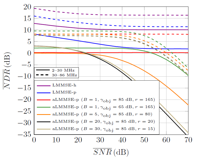
In the considered aLMMSE-p estimators, reducing the rank to the employed values causes no performance loss with respect to their full rank counterparts (although not shown in the figure). However, considerable degradation occurs when using the modeled noise PSD and a fixed [TeX:] $$\gamma_{\mathrm{obj}}$$, especially when the estimator matrix is partitioned into blocks. The comparison of the cases [TeX:] $$\left(B=1,\gamma_{\mathrm{obj}}=85, r=165\right)$$ and [TeX:] $$\left(B=1, \gamma_{\mathrm{obj}}=65, r=165\right)$$ reveals that a lower [TeX:] $$\gamma_{\mathrm{obj}}$$ slighlty improves the performance in the low-mid SNR region at the cost of a significant penalty for high SNR values.
Interestingly, in the 2–30 MHz range, increasing the number of blocks from [TeX:] $$B = 5$$ to [TeX:] $$B = 20$$ and [TeX:] $$B = 30$$ improves the performance in the low SNR region. This is a consequence of the low coherence bandwidth of the channel in this band, which makes the effect of distant carriers to be counterproductive, since the noise they introduce is much larger than the information they provide. However, as the SNR increases, discarding the information from distant carriers cause a severe performance degradation in both frequency bands. It is worth to note that [TeX:] $$B = 20$$ and [TeX:] $$B = 30$$ have quite similar performance values. Further increments in the number of blocks do not cause additional performance degradation because the employed blocks are overlapped 5 carriers, which makes that the response of a given carrier is always estimated using more than 10 carriers.
Fig. 10 depicts the average NDR of the FD-h estimator for different lengths of the sliding window, [TeX:] $$L_{s w}$$. As seen, increasing [TeX:] $$L_{s w}$$ improves the performance in the low SNR region, because of the increased noise reduction, at the cost of reducing the performance in the high SNR region, where the bias introduced by the filtering dominates. In the lower frequency band [TeX:] $$L_{s w}=3$$ seems to be the most appropriate value, while in the high frequency band [TeX:] $$L_{s w}=5$$ provides a good trade-off in the considered SNR range.
Fig. 10.
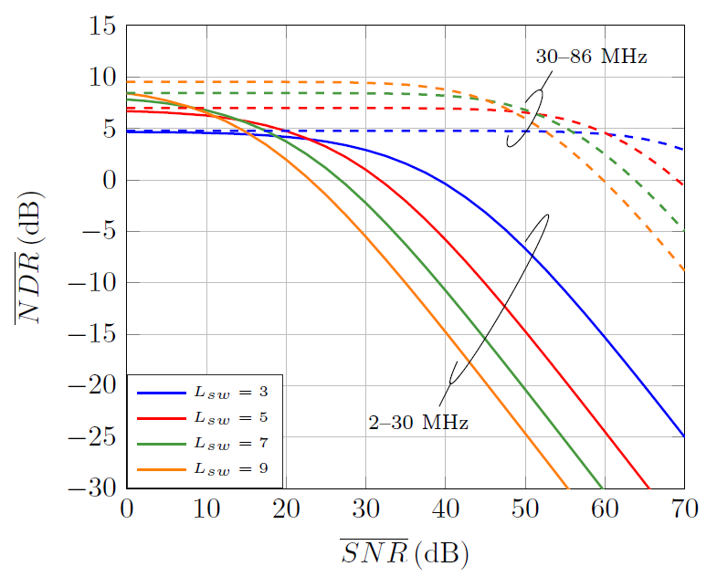
Fig. 11 depicts the average NDR of the DFT-h estimator for different initial and end positions of the non-zero samples that select the MSS of the impulse response. In all cases, the time-domain and frequency-domain shaped regions have [TeX:] $$\beta^h=\alpha^h=10$$ samples. Since most of the MSS of the impulse response are located to the right of the maximum, [TeX:] $$n_a \gt n_b$$ is always selected. As seen, low values of [TeX:] $$n_a+n_b$$ yield higher performance in the low SNR region, because of the increased noise reduction, but cause larger degradation in the high SNR region because of the distortion caused by truncating the impulse response. The NDR degrades when [TeX:] $$n_a+n_b$$ is fixed to a value larger than the effective length of the impulse response because more noise is captured at no benefit. This can be clearly observed by comparing the cases [TeX:] $$\left(n_a=375, n_b=800\right)$$ and [TeX:] $$\left(n_a=375, n_b=1500\right)$$.
Fig. 11.
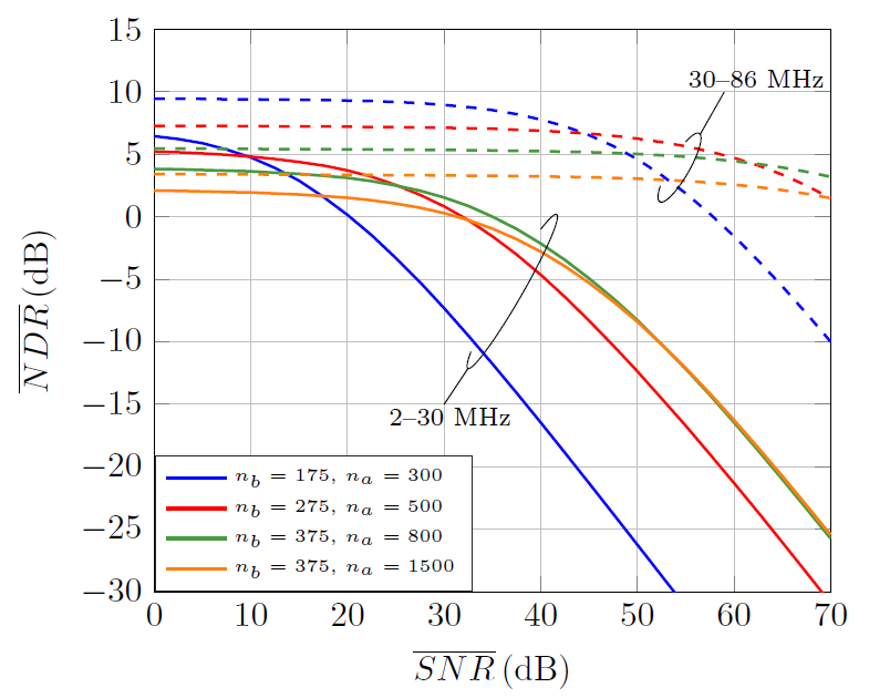
The selection [TeX:] $$\left(n_a=375, n_b=800\right)$$ seems to be the most appropriate one for the low frequency band, while [TeX:] $$\left(n_a=275, n_b=500\right)$$ seems the most suitable for the high frequency region. However, using a different window in the low and high frequency bands would oblige to perform two DFTs as the one in (16), which is impractical because of its high computational cost, as it will be shown in Section V-C. Given that a single window has to be employed, the values [TeX:] $$\left(n_a=375, n_b=800\right)$$ are selected, as in the high frequency band they give NDR values larger than 5 dB in almost the whole SNR range (which ensures that noise will be the limiting factor) and in the low frequency band it gives larger NDR than [TeX:] $$\left(n_a=275, n_b=500\right)$$ in the high SNR region, where estimation errors are the limiting factor.
Fig. 12 shows the average NDR of the estimators designed so far and of the CUB-p, LIN-p and DFT-p ones. In the latter, the frequency-domain shaped region has [TeX:] $$\alpha^p=5$$ samples. As seen, preamble-based estimators perform much worse than the ones based on the header symbol, except for the LMMSE, which performs optimum linear interpolation and smoothing. In the remaining estimators, the additional noise reduction due to the averaging of multiple S1 symbols does not compensate for the distortion introduced by the interpolation. It is worth to note the bad results of the DFT-p estimator, which in a
Fig. 12.
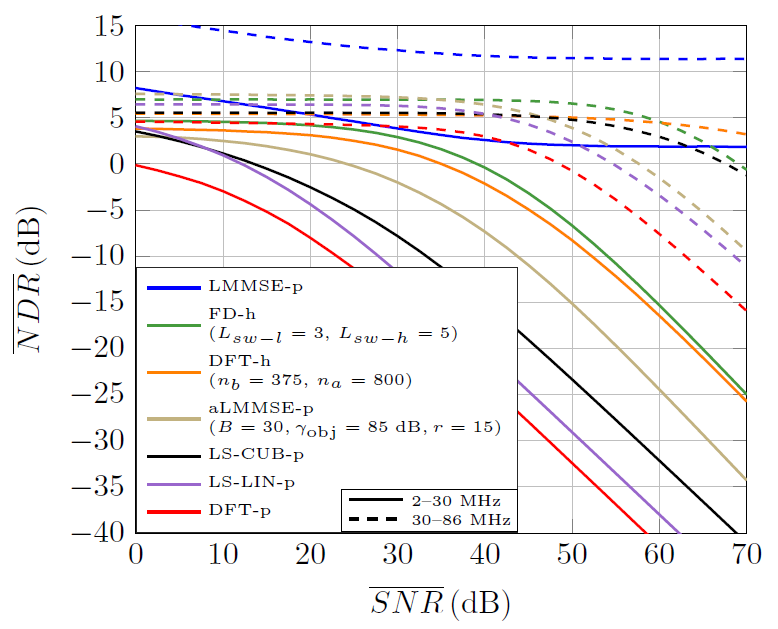
noiseless case without gaps in the bandpass is known to perform optimum interpolation, but gives the worst performance in both frequency bands when the noise is strongly colored noise and the bandpass has multiple notches. Among the practical estimators, in terms of implementation complexity, the FD-h gives the best performance in both bands, except for the SNR region above 60 dB in the 30–86 MHz range, where it is outperformed by the DFT-h estimator. Presented results suggest that, from a channel estimation perspective, the intercarrier spacing used in the preamble is too high and limits the performance of simple interpolation methods.
In order to obtain the combined estimator in (17), results shown in Fig. 12 indicate that the FD-h should be selected to this end because it has higher performance and lower complexity than the DFT-h. For the preamble-based estimation, both the aLMMSE-p with [TeX:] $$\left(B=30, \gamma_{\mathrm{obj}}=85 \mathrm{~dB}, \text { and } \mathrm{r}=15\right)$$ and the CUB-p will be assessed. The aLMMSE-p is selected because of its higher performance and the CUB-p because of its good trade-off between performance and complexity.
Fig. 13 depicts the average NDR of the combined estimators resulting for different values of [TeX:] $$\rho_k$$. Two combination strategies are considered. One in which [TeX:] $$\rho_k=0$$ for [TeX:] $$k \notin 8 \mathbb{N}$$ and [TeX:] $$\rho_k=\rho$$ for [TeX:] $$k \in 8 \mathbb{N}$$, i.e., the header and preamble estimates are effectively combined only in the carriers that are common to the preamble and header symbols. This is denoted as ([TeX:] $$k \in 8 \mathbb{N}$$) in Fig. 13. In the other strategy, [TeX:] $$\rho_k=\rho$$ in all carriers and is labeled as [TeX:] $$(\forall k)$$. The NDR of the constituents estimators (aLMMSE-p, CUB-p and FD-h) are also shown as reference.
Fig. 13.
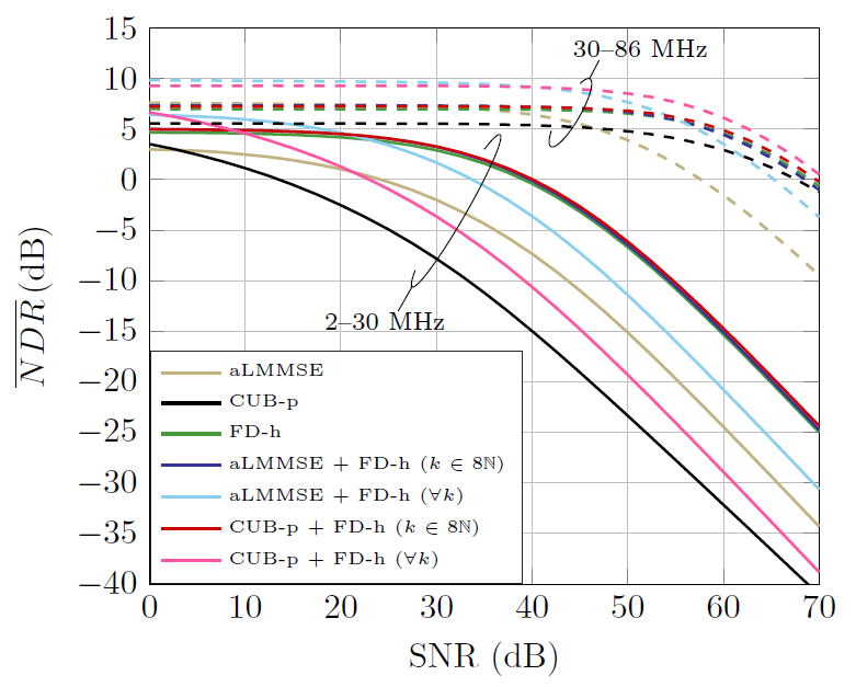
A different value of [TeX:] $$\rho$$ is employed in each frequency band: [TeX:] $$\rho=1$$ in the 2–30 MHz range and [TeX:] $$\rho=3 / 5$$ in the 30–86 MHz band. The rationale for this selection is as follows. Let us focus on the strategy denoted as ([TeX:] $$k \in 8 \mathbb{N}$$). In the 2–30 MHz band, the FD-h estimator reduces the variance of the LS by [TeX:] $$L_{s w}=3 .$$ This is equal to the reduction given by the averaging of the [TeX:] $$M_{S 1}^v=3$$ symbols in the preamble-based estimator, which suggests that [TeX:] $$\rho=1$$ is an appropriate value. In the 30–86 MHz band, since the FD-h estimator reduces the variance of the LS by [TeX:] $$L_{s w}=5, \rho=3 / 5$$ seems more suitable. While this reasoning does not apply to the strategy denoted as [TeX:] $$(\forall k)$$ because of the bias in the preamble-based estimate caused by the interpolation, the performance obtained with the referred values of [TeX:] $$\rho$$ is very close to the optimum one (which has to be determined by simulation).
As shown in Fig. 13, in the 30–86 MHz band, combining the header and preamble estimates in all carriers yields better performance than the strategy that uses [TeX:] $$\rho_k=0$$ for [TeX:] $$k \notin 8 \mathbb{N},$$ resulting in a 2.5 dB gain over the FD-h for [TeX:] $$\mathrm{SNR}\lt 50 \mathrm{~dB}$$. On the contrary, the latter strategy performs better than the former in the 2–30 MHz range. This occurs because the coherence bandwidth of the channel is much lower in the 2–30 MHz than in the 30–86 MHz band, which makes the bias experienced by the preamble-based estimation (due to interpolation) to limit the NDR (instead of the noise) in carriers with indexes [TeX:] $$k \notin 8 \mathbb{N}.$$ It is worth mentioning that, in the 2–30 MHz range, the combination of the preamble and header estimates using the strategy ([TeX:] $$k \notin 8 \mathbb{N}$$) reduces the estimation noise of the involved carriers by about 2.4 dB. However, since this occurs only in 1/8 of the carriers, the resulting average NDR gain over the FD-h is just the 0.3 dB displayed in Fig. 13.
B. Estimators Performance in the Set of Measured Channels
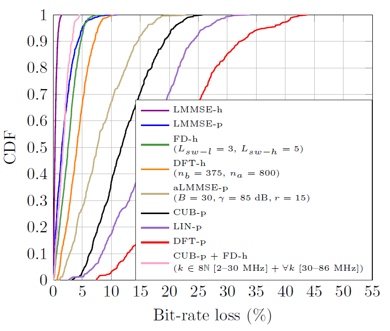
A statistical analysis of the performance of the designed estimators in the set of measured channel responses is now given. To this end, each of the 𝑄 = 171 measured frequency responses is combined with the 4 noise PSD displayed in Fig. 6, yielding 4𝑄 channels. For each one, the bit-rate achieved with the actual channel response and with the one obtained with the considered estimator is computed. The empirical CDF of the bit-rate loss (%) is then computed. To this end, the BPSK to 4096-QAM constellations used in leading PLC systems subject to an objective bit-error probability of [TeX:] $$10^{-5}$$ are employed. Uncoded transmission is considered to prevent the channel coding from hindering the actual performance differences among estimators and to make results independent of the considered system, since different channel codes are defined in the ITU-T G.hn (LDPC) and the IEEE P1901 and HomePlug AV2 (turbo code). The estimation error is assumed to be Gaussian, which yields a lower bound on the performance. The injected signal uses the maximum PSD values defined in the ITU-T Rec. G9964 [10]. The pre-computed matrix of the aLMMSE estimators is always obtained using the modeled PSD corresponding to Noise 3 in Fig. 6. The estimators are configured using the same parameters as in Fig. 12. The combined estimator employes the ([TeX:] $$k \in 8 \mathbb{N}$$) strategy with [TeX:] $$\rho=1$$ in the 2–30 MHz band and the [TeX:] $$(\forall k)$$ strategy with [TeX:] $$\rho=3 / 5$$ in the 30–86 MHz range. Only the combined estimator based on the CUB-p is shown because it performs similarly to the one based on the aLMMSE-p but has lower complexity.
Results obtained are depicted in Fig. 14. As seen, the LMMSE-h offers the lower bit-rate loss, with a maximum value about 1.5%. Interestingly, the CUB-p + FD-h performs very close to the LMMSE-h, giving a maximum bit-rate loss of 4.5%. The LMMSE-p perform marginally better than the CUB-p + FD-h in 60% of the channels but worse in the remaining 40%. The good performance of the LMMSE-p indicates that the mismatch due to the use of estimated channel correlation matrices is negligible. Among the estimators that operate exclusively over the header symbol, the FD-h gives better performance than the DFT-h one, with maximum bit-rate loss of 9% and 10.5%, respectively. Regarding the estimators that operate over the preamble symbols, the aLMMSE gives the best performance. The DFT-p is the worst, mainly due to the undersampling in frequency that occurs because of the low intercarrier spacing used in the preamble symbols, which causes time aliasing.
Fig. 14.
C. Computational Complexity
Table III summarizes the number of complex products and sums required to implement the presented estimators, whose details are given in the appendix. The number of passband notched carriers of the header and preamble symbols are denoted as [TeX:] $$N_h^{\text {notch }}$$ and [TeX:] $$N_p^{\text {notch }}$$, respectively; [TeX:] $$N_{h-l}^a$$ and [TeX:] $$N_{h-h}^a$$ denote the number of active carriers of the header symbol in the 2–30 MHz and 30–86 MHz bands, respectively. In the aLMMSE-p estimator, [TeX:] $$N_h(b)$$ and [TeX:] $$N_p(b)$$ denote the number of header and preamble carriers in the 𝑏th block. Note that due to the notches in the passband and to the fact that [TeX:] $$N_h^a$$ and [TeX:] $$N_p^a$$ will not be generally multiple of the number of blocks, [TeX:] $$B$$, the number of carriers may slightly vary among blocks and so does the corresponding rank [TeX:] $$r(b)$$. The term [TeX:] $$N_p^{o v l p}(b)$$ denotes the number of carriers of the 𝑏th block that overlap with the adjacent blocks. Hence, [TeX:] $$N_p^{o v l p}(1)=N_p^{o v l p}(B)=5 \text {, }$$ because there is no preceding/subsequent block, and [TeX:] $$N_p^{o v l p}(b)=10$$ in the remaining ones.
TABLE III
| Estimator | Number of complex products | Number of complex sums |
|---|---|---|
| FD-h | [TeX:] $$2 N_h^a+N_h^{n o t c h}$$ | [TeX:] $$2 N_h^{\text {notch }}+\left(L_{s w-l}-1\right) N_{h-l}^a+\left(L_{s w-h}-1\right) N_{h-h}^a$$ |
| DFT-h | [TeX:] $$N_h^a+N_h^{\text {notch }}+2\left(\beta^h+\alpha^h\right)+N_h \log _2\left(N_h\right)$$ | [TeX:] $$2 N_h^{\text {notch }}+2 N_h \log _2\left(N_h\right)$$ |
| aLMMSE-p | [TeX:] $$N_p^a+\sum_{b=1}^B r(b)\left[N_h(b)+N_p(b)+N_p^{o v l p}(b)\right]$$ | [TeX:] $$M_{S 1}^{\mathrm{v}} N_p^a+\sum_{b=1}^B r(b)\left[N_h(b)+N_p(b)+N_p^{o v l p}(b)-1\right]$$ |
| CUB-p | [TeX:] $$N_p^a+N_p^{\text {notch }}+13\left(N_h^a-N_p^a\right)$$ | [TeX:] $$M_{S 1}^{\mathrm{v}} N_p^a+2 N_p^{\text {notch }}+14\left(N_h^a-N_p^a\right)$$ |
| LIN-p | [TeX:] $$N_p^a+\left(N_h^a-N_p^a\right)$$ | [TeX:] $$M_{S 1}^{\mathrm{v}} N_p^a+2\left(N_h^a-N_p^a\right)$$ |
| DFT-p | [TeX:] $$N_p^a+N_p^{\text {notch }}+2 \alpha^p+\left(N_p / 2\right) \log _2\left(N_p\right)+\left(N_h / 2\right) \log _2\left(N_h\right)$$ | [TeX:] $$M_{S 1}^{\mathrm{v}} N_p^a+2 N_p^{\text {notch }}+N_p \log _2\left(N_p\right)+N_h \log _2\left(N_h\right)$$ |
Fig. 15 depicts the values obtained when evaluating the expressions in Table III. Estimators are configured with the same parameters employed in Fig. 14. Interestingly, the FD-h, which has been shown to give excellent performance, is almost the simplest one (except for the LIN-p). It must be recalled that header-based techniques require the header symbol to be correctly decoded, for which a preamble-based estimator has to be employed. Nevertheless, since the header bits are strongly coded and modulated using QPSK, the performance of the employed estimator can be lower than the one used for the payload symbols, which may use constellations up to 1024 QAM. The incremental complexity of the combined estimator with respect to the FD-h is just [TeX:] $$N_{h-l}^a / 8+2 N_{h-h}^a$$ products and [TeX:] $$N_{h-l}^a / 8+N_{h-h}^a$$ sums.
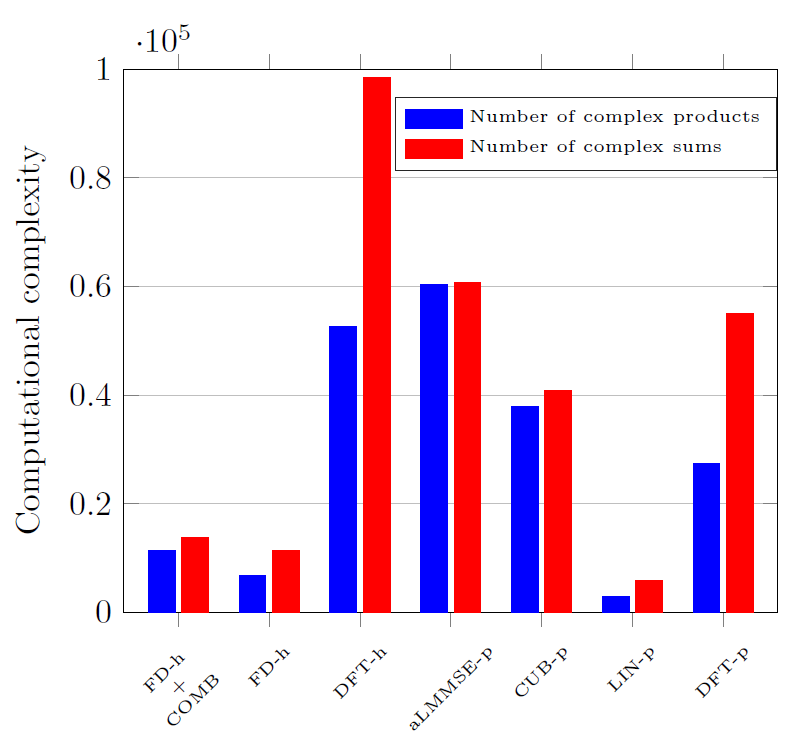
The DFT-h estimator, which also gives a good estimation performance, is the most complex method in terms of number of sums and the second one in terms of number of products because of the high cost of the [TeX:] $$N_h \text {-samples }$$ IDFT and DFT. Among the preamble-based estimators, the aLMMSE-p offers the best performance but is also the most complex one.
The complexity of the LMMSE-h and the LMMSE-p (not shown in the figure) is about 22 and 180 times larger than the one of the aLMMSE-p, respectively, even without taking into account the cost associated to compute the estimator matrix (which requires a matrix sum, a matrix inversion and a matrix product).
VI. CONCLUSION
This work has addressed the problem of channel estimation in state-of-the-art indoor PLC systems in the frequency band up to 100 MHz. To this end, the relevant characteristics of PLC channels for the considered problem have been firstly reviewed. The distinctive features of PLC channels with respect to wireless ones, especially its non-ergodic nature and the absence of fading, and their implications in channel estimation methods that require knowledge of the channel statistics is discussed.
Several channel estimation techniques are then presented and their most appropriate parameters for PLC channels are derived. The trade-off between bias and variance is discussed. This arises because estimations from the preamble can benefit from the noise reduction given by the averaging of estimates from multiple symbols, but suffer larger bias caused by interpolation, as intercarrier spacing in the preamble symbols is larger than in the header and payload ones.
A statistical analysis of the performance of the presented estimation techniques in a large set of measured PLC channels and an assessment of their computational complexity is given. Results indicate that estimators based on the header symbol give higher performance than preamble-based ones and that nearly optimum performance can be achieved by using a computationally simple estimator that combines the estimations obtained from both type of symbols.
APPENDIX
This appendix details the operations that yield the computational costs summarized in Table III. The following assumptions are made: An 𝑁-samples DFT/IDFT requires [TeX:] $$(N / 2) \log _2(N)$$ products and [TeX:] $$N \log _2(N)$$ sums; piecewise cubic interpolation requires 13 products and 14 sums per interpolated point when implemented as in [34]; piecewise linear interpolation requires one product and two sums (assuming that the slopes of the lines in (11) are precomputed, which is feasible because they correspond to known positions). Regarding the computation of the LS estimates: the cost of the DFTs are not included because the one of the header symbol has been previously computed to decode it and the ones of the preamble symbols are also required for other purposes such as sampling and carrier frequency offset estimation; in the preamble, the division by the constellation symbols can be implemented as a product because they are predefined (including the division by [TeX:] $$M_{S 1}^{\mathrm{v}}$$), while in the header symbol it requires two products when implemented as [TeX:] $$1 / x^s(k)=x^s(k)^* /\left|x^s(k)\right|^2$$, where [TeX:] $$1 /\left|x^s(k)\right|^2$$ is precomputed.
The FD-h method has three steps: the computation of the LS, the linear interpolation of the channel response in the notched carriers and the smoothing using the sliding window. The LS requires one product and is computed in [TeX:] $$N_h^a$$ values. The interpolation requires [TeX:] $$N_h^{\text {notch }}$$ products and [TeX:] $$2 N_h^{\text {notch }}$$ sums, since the slope of the linear interpolation can be precomputed. The sliding window filtering in (12) requires one product and [TeX:] $$L_{s w}-1$$ sums per output value. It is applied to obtain [TeX:] $$N_{h-l}^a$$ output values with a sliding window of length [TeX:] $$L_{s w-l}$$ and [TeX:] $$N_{h-h}^a$$ ones with a window of length [TeX:] $$L_{s w-h}$$, being [TeX:] $$N_h^a=N_{h-l}^a+N_{h-h}^a.$$
The DFT-h consists of an IDFT and a DFT with joint cost of [TeX:] $$N_h^a \log _2\left(N_h^a\right)$$ products and [TeX:] $$2 N_h^a \log _2\left(N_h^a\right)$$ sums; the product by the [TeX:] $$\mathbf{S}^h$$ window in (15) and [TeX:] $$\mathbf{w}^h$$ in (16), which have [TeX:] $$\alpha^h$$ and [TeX:] $$\beta^h$$ tapered samples at each side, respectively, and the interpolation required to compute the channel response in the [TeX:] $$N_h^{\text {notch }}$$ notched carriers.
The first term of the number of products and sums of the aLMMSE-p in Table III is due to the averaging of the [TeX:] $$N_p^a$$ channel response values obtained in [TeX:] $$M_{S 1}^{\mathrm{v}}$$ symbols, which requires [TeX:] $$M_{S 1}^{\mathrm{v}} N_p^a$$ sums and one product by the inverse of [TeX:] $$M_{S 1}^{\mathrm{v}}$$. This term is common to all preamble-based estimation techniques. The second term is due to the core operations of the aLMMSE-p, which is taken from [13, Appendix C].
The second term in the number of products and sums of the CUB-p and the DFT-p methods in Table III corresponds to the interpolation of the frequency response in the notched carriers. The third term of the CUB-p and the second in LIN-p are due to the interpolation required to determine the frequency response in the [TeX:] $$N_h^a-N_p^a$$ data carriers not transmitted in the preamble symbols.
The third term of the number of products and sums of the DFT-p method in Table III corresponds the product by the [TeX:] $$\mathbf{S}^p$$ window in (13), which has [TeX:] $$\alpha^p$$ tapered samples at each side. The two last terms correspond to the cost of the [TeX:] $$N_p \text {-samples }$$ IDFT and the [TeX:] $$N_h \text {-samples }$$ DFT, respectively.
Biography
José A. Cortés
José A. Cortés received the M.S. and Ph.D. degrees in Telecommunication Engineering from the Universidad de Málaga, Spain, in 1998 and 2007, respectively. In 1999, he was with Alcatel España RD. He joined the Communication Engineering Department, Universidad de Málaga, in 1999, where he became an Associate Professor in 2010. From 2000 to 2002, he collaborated with the Nokia System Competence Team in Málaga. From 2014 to 2016 he was on a leave of absence working as a Consultant on the Development of Atmel’s Power Line Communications (PLC) Solutions. He was the General Co-Chair of the IEEE ISPLC 2020. He is Associate Editor of the IEEE Open Journal of the Communications Society, where he has been recognized as Exemplary Editor in 2021. He served as Associate Editor of the IEEE Communications Letters, where he has been recognized as Exemplary Editor in 2019, 2020 and 2021. He serves as Chair of the IEEE Communications Society Technical Committee on Power Line Communications since 2022. His research interests include digital signal processing for communications, mainly focused on channel characterization and transmission techniques for PLC.
References
- 1 L. T. Berger, A. Schwager, P. Pagani, and D. M. Scheneider, Eds.,MIMO power line communications: Narrow and broadband standards, EMC and avanced processing, 1st ed. Boca Raton, FL: CRC Press, 2014.doi:[[[10.1201/b16540]]]
- 2 S. Aboagye, T. M. N. Ibrahim, A. Ngatched, A. R. Ndjiongue, and O. A. Dobre, "Design of energy efficient hybrid VLC/RF/PLC communication system for indoor networks,"IEEEWirelessCommun.Lett., vol. 9, no. 1, pp. 143-147, Feb. 2020.doi:[[[10.1109/LWC.2019.2946144]]]
- 3 K. Ali, A. X. Liu, I. Pefkianakis, and K. H. Kim, "Distributed spectrum sharing for enterprise powerline communication networks," IEEE/ACM Trans. Netw., vol. 29, no. 3, pp. 1032-1045, Jun. 2021.doi:[[[10.1109/TNET.2021.3056512]]]
- 4 G. López et al., "The role of power line communications in the smart grid revisited: Applications, challenges, and research initiatives," IEEE Access, vol. 7, pp. 117346-117368, Jul. 2019.doi:[[[10.1109/ACCESS.2019.2928391]]]
- 5 L. Lampe, A. M. Tonello, and T. G. Swart, Eds., Power line communications: Principles, standards and applications from multimedia to Smart Grid, 2nd ed. Wiley, Jun. 2016.custom:[[[https://www.wiley.com/en-be/Power+Line+Communications%3A+Principles%2C+Standards+and+Applications+from+Multimedia+to+Smart+Grid%2C+2nd+Edition-p-9781118676714]]]
- 6 G. Hallak, M. Berners, and A. Mengi, "Planning approach towards optimal performance and cost of G.hn broadband PLC access networks," in IEEE ISPLC, 2020.doi:[[[10.1109/ISPLC48789.2020.9115399]]]
- 7 "Unified high-speed wireline-based home networking transceivers system architecture and physical layer specification," ITU-T Recommendation G.9960, International Telecommunications Union, Jul. 2015.custom:[[[-]]]
- 8 "Data link layer (DLL) for unified high-speed wire-line based home networking transceivers," ITU-T Recommendation G.9961, International Telecommunications Union, Jun. 2010.custom:[[[-]]]
- 9 "Unified high-speed wireline-based home networking transceivers multiple input/multiple output specification," ITU-T Recommendation G.9963, International Telecommunications Union, Dec. 2011.custom:[[[-]]]
- 10 "Unified high-speed wireline-based home networking transceivers power spectral density specification," ITU-T Recommendation G.9964, International Telecommunications Union, Dec. 2011.custom:[[[https://standards.globalspec.com/std/10019935/itu-t-g-9964]]]
- 11 IEEE Std 1901-2020, "IEEE standard for broadband over power line networks: Medium access control and physical layer specifications."custom:[[[-]]]
- 12 "HomePlug A V specification version 2.1," HomePlug Alliance, Specification. (Online). Available: https://bit.ly/39YvjXB, Feb. 2014.custom:[[[https://bit.ly/39YvjXB,Feb.2014]]]
- 13 O. Edfors, M. Sandell, J. J. van de Beek, S. K. Wilson, and P. O. Börjesson, "OFDM channel estimation by singular value decomposition," IEEE Trans. Commun., vol. 46, no. 7, pp. 931-939, Jul. 1998.doi:[[[10.1109/VETEC.1996.501446]]]
- 14 A. T. Asyhari, "New bounds on the mutual information for discrete constellations and application to wireless channel estimation," Digit. Commun. Netw., vol. 6, no. 4, pp. 542-546, 2020.custom:[[[-]]]
- 15 S. M. Kay, Fundamentals of statistical signal processing: Estimation theory. Prentice Hall, 1993.custom:[[[-]]]
- 16 D. Bueche, P. Corlay, M. Gazalet, and F.-X. Coudoux, "A method for analyzing the performance of comb-type pilot-aided channel estimation in power line communications," IEEE Trans. Consum. Electron., vol. 54, no. 3, pp. 1074-1081, Aug. 2008.custom:[[[-]]]
- 17 O. Edfors, M. Sandell, J. J. van de Beek, S. K. Wilson, and P. O. Börjesson, "Analysis of DFT-based channel estimators for OFDM," Wireless Pers. Commun., vol. 12, no. 1, pp. 55-70, 2000.custom:[[[-]]]
- 18 S. Rosati, G. E. Corazza, and A. Vanelli-Coralli, "OFDM channel estimation based on impulse response decimation: Analysis and novel algorithms,"IEEETrans.Commun., vol. 60, no. 7, pp. 1996-2008, 2012.custom:[[[-]]]
- 19 C. R. Paul, Analysis of multiconductor transmission lines. New Jersey: John Wiley Sons, 1994. MHzcustom:[[[-]]]
- 20 M. Colombo, A. Hernández, and J. Ureña, "Low-complexity joint time synchronization and channel estimation for OFDM-based PLC systems," IEEE Access, vol. 7, pp. 121446-121456, 2019.custom:[[[-]]]
- 21 J. Huang, P. Wang, and Q. Wan, "Robust approach for channel estimation in power line communication," J. Commun. Netw., vol. 14, no. 3, pp. 237-242, Jun. 2012.custom:[[[-]]]
- 22 Y .-R. Chien, "Iterative channel estimation and impulsive noise mitigation algorithm for OFDM-based receivers with application to powerline communications," IEEE Trans. Power Del., vol. 30, no. 6, pp. 2435-2442, Dec. 2015.custom:[[[-]]]
- 23 D. Shrestha, X. Mestre, and M. Payaró, "On channel estimation for power line communication systems in the presence of impulsive noise," Comput. Elect. Eng., vol. 72, pp. 406-419, Nov. 2018.custom:[[[-]]]
- 24 R. Shaked, N. Shlezinger, and R. Dabora, "Joint estimation of carrier frequency offset and channel impulse response for linear periodic channels," IEEE Trans. Commun., vol. 66, no. 1, pp. 302-319, Jan. 2018.custom:[[[-]]]
- 25 D. Altolini, N. Benvenuto, S. Pupolin, and R. Riva, "Preamble-based channel estimation in HomePlug A V systems," in IEEE ISPLC, 2012.custom:[[[-]]]
- 26 J. A. Cortés et al., "Feasibility study of power line communications for backhauling outdoor small cells,"IEEEAccess, vol. 9, pp. 30135-30153, Feb. 2021.custom:[[[-]]]
- 27 F. J. Cañete, J. A. Cortés, L. Díez, and J. T. Entrambasaguas, "Modeling and evaluation of the indoor power line channel," IEEE Commun. Mag., vol. 41, no. 4, pp. 41-47, Apr. 2003.custom:[[[-]]]
- 28 F. J. Cañete, J. A. Cortés, L. Díez, and J. T. Entrambasaguas, "A channel model proposal for indoor power line communications," IEEE Commun. Mag., vol. 49, no. 12, pp. 166-174, Dec. 2011.custom:[[[-]]]
- 29 F. J. Cañete, J. A. Cortés, L. Díez, and J. T. Entrambasaguas, "Analysis of the cyclic short-term variation of indoor power line channels," IEEE J. Sel. Areas Commun., vol. 24, no. 7, pp. 1327-1338, Jul. 2006.custom:[[[-]]]
- 30 J. A. Cortés, L. Díez, F. J. Cañete, and J. J. Sánchez-Martínez, "Analysis of the indoor broadband power-line noise scenario," IEEE Trans. Electromagn. Compat., vol. 52, no. 4, pp. 849-858, Nov. 2010.custom:[[[-]]]
- 31 T. Esmailian, F. R. Kschischang, and P. G. Gulak, "In-building power lines as high-speed communication channels: Channel characterization and a test channel ensemble," International J. Commun., vol. 16, pp. 381-400, Jun. 2003.custom:[[[-]]]
- 32 A. M. Tonello, F. Versolatto, and A. Pittolo, "In-home power line communication channel: Statistical characterization," IEEE Trans. Commun., vol. 62, no. 2, pp. 2096-2106, 2014.custom:[[[-]]]
- 33 T. Bai et al., "Fifty years of noise modeling and mitigation in powerline communications," IEEE Commun. Surveys Tuts., vol. 23, no. 1, pp. 41-69, 2021.custom:[[[-]]]
- 34 R. G. Keys, "Cubic convolution interpolation for digital image processing," IEEE Trans. Acoust., Speech, Signal Process., vol. ASSP-29, no. 6, pp. 1153-1160, 1981.custom:[[[-]]]
- 35 H. Minn and V . K. Bhargava, "An investigation into time-domain approach for OFDM channel estimation," IEEE Trans. Broadcasting, vol. 46, no. 4, pp. 240-248, 2000.custom:[[[-]]]