Fedor Ivanov , Valerii Morishnik and Evgenii Krouk
Improved Generalized Successive Cancellation List Flip Decoder of Polar Codes with Fast Decoding of Special Nodes
Abstract: In this paper, an improvement for SC list flip (SCLFlip) decoding is presented for polar codes. A novel bit-selection metric for critical set (set of information symbols of polar codes being flipped during additional decoding attempts) based on path metric of successive cancellation list (SCL) decoding is suggested. With the proposed metric, the improved SCL scheme based on special nodes (SN) decoders was developed. This decoder will be denoted by GSCLF. The main idea of the proposed decoder is joint using of two approaches: first one is a fast decoding of special nodes in binary tree representation of polar code (e.g., some special nodes in tree representation of polar code that allow efficient list decoding with low complexity) and the second one is an applying of additional decoding attempts (flips) in the case when initial decoding was erroneous. The simultaneous use of these two approaches results in both a significant reduction in spatial complexity and a significant reduction in the number of computations required for decoding whereas keeping excellent performance. Simulation results presented in this paper allow us to conclude that the computational complexity of the proposed GSCLF decoder is from 66% to 80% smaller than the one of SCL-32 decoder.
Keywords: polar codes , scl-flip decoding , subcodes of polar code , successive cancellation list decoding
I. INTRODUCTION
Arikan firstly proved that polar codes could achieve the capacity of any symmetric binary input symmetric discrete memoryless channels (B-DMCs) under a successive cancellation (SC) decoder as the code length goes to infinity [1].
Unfortunately, for short and moderate code length, the error rate performance of SC decoding for polar codes is inferior to LDPC and turbo codes. As an enhanced version of SC, the SC list (SCL) decoder [2] searches the code tree level by level, in much the same manner as SC. However, SCL allows a maximum of L candidate paths to be further explored, which preserves the further error correction ability.
Cyclic redundancy check (CRC)-aided SCL (CA-SCL) decoding scheme is a kind of SCL decoder, which outputs the SCL candidate paths into a CRC detector, and the check results are utilized to detect the correct codeword [3].
There are some special cases when it is not required to traverse all tree for SC/SCL decoding. More precisely, there are special nodes in tree representation of polar code that can be decoded directly with complexity significantly lower than direct SC application. This approach is known as simplified SC decoding [4]. It was followed by fast-SSC decoding [5] and several others to reduce the latency of SC decoding [6].
It was further extended to simplified SCL, with reduced latency and more practical implementation potential [7]. For simplified SCL, the number of operations can be reduced from 2.8 to 4.32 times in comparison with conventional SCL for length N = 1024 polar code with different rates [8].
Simplified decoding is one of the most promising approaches when it is required to significantly decrease a number of decoding operations i.e., to decrease decoding latency. On the other hand the performance of this approach in terms of frame error rate is approximately the same as for SC or SCL. At the same time these fast decoding techniques for polar codes are known for their significantly added space complexity and power consumption [9].
Bit-flipping approach is aimed to solve the problem of space complexity of SCL decoding. SC-flip (SCF) decoding algorithm was first presented in [10]. The main idea of SCF is to use additional SC decoding attempts in series in the case when an initial SC decoding fails due to a single channelinduced error. The first paper where SCL decoding with flips (SCLF) was presented is [11]. In this paper we will show how the same flipping approach can be adapted for simplified SCL decoding to reduce it’s space complexity and power consumption.
One of the most important differences between various SC/SCL decoders with flips is the way to construct critical set (CS). During the course of the initial SC/SCL decoding, a CS of T bit-flipping indices [TeX:] $$\mathcal{F}_{\text {inv }}=\left\{i_{1}, i_{2}, \cdots, i_{T}\right\}$$ are calculated and stored based on a selection criterion f. There are a lot of papers where authors try to improve performance of SCF/SCLF by considering more advanced methods for CS construction. The present work is mainly based on approach to construct CS presented in [12]. SNR dependent approach to design CS was proposed in [13]. CS design based on deep learning of LSTM recurrent neural network was proposed in [14]. Shifted pruning approach for CS constructing was discussed in [15] and [16]. Shifted pruning based CS can be obtained offline.
There are some other approaches that allow to improve performance of SCF/SCLF. Multiple bit-flipping was proposed in [17]. Instead of single flipping (one information bit per each additional decoding attempt) this approach implies several (usually not more than 4) flips during each extra decoding. In paper [18] dynamic SCF decoding (DSCF) was introduced. This decoder on the one hand allows multiple flips and on the other hand Finv is recalculated after each failed decoding attempt. This approach is more powerful and it was shown that DSCF decoding with T = 50 single flips has the same performance as SCL-8 and T = 400 flips allow to reach performance of SCL-16 for (1024; 512) polar code with CRC-16. Multiple bit-flipping with nested construction of CS can further improve performance of SC decoding. Nested CS approach was also proposed in [17] and simulation results from this paper show that applying 4-level CS construction jointly with SCF decoding results in approximately the same performance as SCL-32 for (1024; 512) polar code with CRC-24. An improved segmented flipped successive cancellation list (ISFSCL) decoder, with a reasonable segmentation strategy and a number of extra flipping attempts was proposed in [19].
Most existing SCLF decoders operate with symbols of the received word instead of some patterns of symbols (special nodes) that can be decoded directly without tree traversing. In this paper we propose new improved generalized bitflipping decoding (GSCLF) of polar codes that is aimed to solve two problems simultaneously: Reducing both space and computational complexities in comparison with SCL. Here term “generalized” means that this decoder involves fast decoders of special/generalized nodes of polar code. First issue is solved due to additional decoding attempts that allow to reduce list size. The second one is resolved by applying simplified version of SCL that reduces number of operations. To realize our decoder we additionally suggest novel method of CS construction that can be applied both for symbol-wise and generalized SCL decoders.
II. PRELIMINARY INFORMATION
In this paper we use standard notation: for any vector [TeX:] $$\mathrm{V}= \left(v_{0}, \cdots, v_{N-1}\right)$$ under [TeX:] $$\mathbf{v}_{i}^{j}$$ we understand [TeX:] $$\left(v_{i}, v_{i+1}, \cdots, v_{j}\right).$$
A. Polar Codes
Polar codes are rooted in the channel polarization phenomenon. At first, the same independent channels are transformed into two kinds of synthesized sub-channels: more reliable channels and less reliable channels. By recursively applying such polarization transformation, when the code length is sufficient, the synthesized sub-channels converge to two extreme groups: The noisy sub-channels and almost noise-free sub-channels. Since the noiseless channels have higher capacities/reliabilities than the noisy channels, polar codes transmit information bits over the noiseless sub-channels while assigning frozen bits (fixed value of zeroes or ones, and assumed known at both the encoder and decoder) to the noisy ones.
However, for finite code length N, the polarization of the sub-channels is incomplete. Sub-channels with different
Fig. 1.
reliabilities are in between the noiseless (high reliability) subchannels and noisy (low reliability) sub-channels. To choose a subset [TeX:] $$\mathcal{I}$$ of K sub-channels from [TeX:] $$\{0,1, \cdots, N-1\}$$ to encode K information bits becomes the polar code construction problem. Here N is restricted to powers of two [TeX:] $$\left(N=2^{n},\right. n \geq 0),$$ and the complement of [TeX:] $$\mathcal{I}$$ in [TeX:] $$\{0,1, \cdots, N-1\}$$ is called frozen sub-channels which denoted as [TeX:] $$\mathcal{F},$$ i. e. [TeX:] $$\mathcal{F}=\mathcal{I}^{c}=\{0,1, \cdots, N-1\} \backslash \mathcal{I}.$$
Consider a binary (N,K) polar code specified by set [TeX:] $$\mathcal{I}$$ of information indexes, set of frozen indexes [TeX:] $$\mathcal{F}=\mathcal{I}^{c},|\mathcal{I}|=K, |\mathcal{F}|=N-K, N=2^{n}, n \in \mathbb{N} and the corresponding encoding procedure:$$
where [TeX:] $$\mathrm{d} \in\{0,1\}^{N} \text { and } \mathrm{G}_{N}$$ is the generator matrix of order N, defined as [TeX:] $$\mathbf{G}_{N}=\mathbf{F}^{\otimes n}$$ with the Arikan’s standard polarizing kernel [TeX:] $$\mathbf{F} \triangleq\left[\begin{array}{ll} 1 & 1 \\ 0 & 1 \end{array}\right] \text { and } \otimes n$$ is n-fold Kronecker product of F.
We consider the frozen bits as zeroes, [TeX:] $$\mathrm{d}_{\mathcal{F}}=0,$$ and the information bits as the information to be encoded, [TeX:] $$\mathrm{d}_{\mathcal{I}}=\mathrm{u}.$$
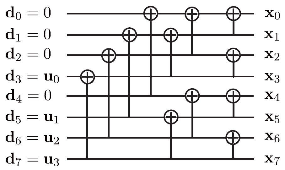
Fig. 1 illustrates an encoding example with polar code (8,4), where information set is [TeX:] $$\mathcal{I}=\{0,1, \cdots, N-1\}.$$
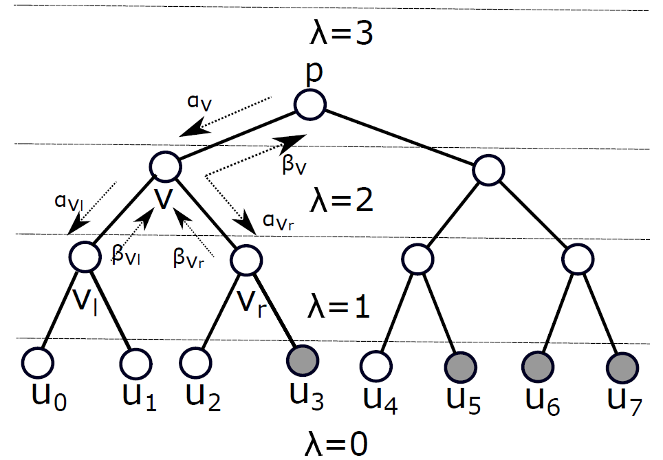
For our purposes it is more convenient to consider polar code as a binary tree where leaf nodes correspond to code symbols. Tree structure of described above (8,4) polar code [TeX:] $$(\mathcal{I}=\{3,5,6,7\})$$ is presented in Fig. 2 where filled circles at last level [TeX:] $$\lambda=0$$ correspond to information symbols and empty ones to frozen symbols. Also it can be noticed from the picture that length N polar code correspond to [TeX:] $$\log _{2} N+1$$ levels (enumerated from leafs to root p) in the tree and each node in i-th subtree can be assumed as length [TeX:] $$2^{i}$$ subcode of polar code which in fact is also a polar code.
Both encoding and decoding of polar code can be described in terms of recursive application of [TeX:] $$(u+v, v)$$ Plotkin construction in the tree. Encoder starts at level [TeX:] $$\lambda=0$$ and applies [TeX:] $$(u+v, v)$$ for each pair of symbols [TeX:] $$\left(u_{0}, u_{1}\right), \left(u_{2}, u_{3}\right), \cdots,\left(u_{N-2}, u_{N-1}\right)$$ to obtain N=2 codewords [TeX:] $$\mathbf{u}_{0}^{(1)}, \mathbf{u}_{1}^{(1)}, \mathbf{u}_{2}^{(1)}, \cdots, \mathbf{u}_{N / 2}^{(1)}$$ of length 2 polar codes. Then these vectors divide into pairs [TeX:] $$\left(\mathbf{u}_{0}^{(1)}, \mathbf{u}_{1}^{(1)}\right), \cdots,\left(\mathbf{u}_{N / 2-2}^{(1)}, \mathbf{u}_{N / 2-1}^{(1)}\right)$$ and Plotkin construction is applied to each of these pairs to obtain N=4 codewords of length 4 polar codes at level [TeX:] $$\lambda=2$$ etc. This process terminates when [TeX:] $$(u+v, v)$$ applies to two N=2-length vectors at level [TeX:] $$\lambda=\log N-1.$$ The result of transform is codeword of (N,K) polar code with information set [TeX:] $$\mathcal{I}$$.
B. Successive Cancellation Decoding
The SC decoding algorithm can be regarded as a greedy search algorithm over the compact-stage code tree described above. Between the two branches associated with an information bit at a certain level, only the one with the larger probability is selected for further processing. Whenever a bit is wrongly determined, correcting it in future decoding procedures becomes impossible.
Also SC decoder might be considered as a special type of message-passing decoding where messages passed along edges that connect parent nodes with their children.
The general aim of SC decoding is to estimate [TeX:] $$\hat{u}_{0}^{K-1}$$ for all information symbols. Since SC is sequential decoding, then ith information bit is decoded under the assumption that all previous information bits were correctly recovered:
(2)
[TeX:] $$\hat{u}_{i}=\left\{\begin{array}{l} \underset{u_{i} \in\{0,1\}}{\arg \max } W_{n}^{(i)}\left(\mathbf{y}_{0}^{N-1}, \hat{\mathbf{u}}_{0}^{i-1} \mid u_{i}\right), \text { if } i \in \mathcal{I} \\ 0, \text { otherwise } \end{array}\right.$$where [TeX:] $$\mathbf{y}_{0}^{N-1}=\left(y_{0}, y_{1}, \cdots, y_{N-1}\right) -$$ received from channel vector of log-likelihoods: [TeX:] $$y_{i} \triangleq \ln \frac{W\left(y_{i} \mid x_{i}=0\right)}{W\left(y_{i} \mid x_{i}=1\right)},$$ where [TeX:] $$W(y \mid x), x \in\{0,1\}, y \in \mathbb{R}$$ is a channel transition probability function and [TeX:] $$W_{n}^{(i)}\left(\mathbf{y}_{0}^{N-1}, \hat{\mathbf{u}}_{0}^{i-1} \mid u_{i}\right)$$ represents the likelihood of [TeX:] $$u_{i}$$ given the channel output [TeX:] $$\mathrm{y}_{0}^{N-1} \text { and } \hat{\mathrm{u}}_{0}^{i-1}$$ considering [TeX:] $$\mathbf{u}_{i+1}^{N-1}$$ as unknown bits.
C. Successive Cancellation List Decoding
As an enhanced version of SC, the SCL decoder [2] searches the code tree level by level, in much the same manner as SC. However, SCL allows a maximum of L candidate paths to be further explored, which preserves the further error correction ability.
SCL decoding maintains L concurrent decoding candidates. In order to construct these candidates [TeX:] $$\hat{u}_{i}$$ at leaf nodes is estimated as both 0 and 1 when not being a frozen bit, doubling the number of candidates (paths). To estimate the reliability of each path during the decoding process and limit the number of possible candidates path metric (PM) is used. PM limits the exponential increase of complexity: When number of paths become higher than list size L, then only L paths with minimal PM are preserved and other paths are eliminated. There are different approaches to construct PM. The most widely-used and hardware-friendly approach for PM calculation proposed in [20].
where [TeX:] $$l=1, \cdots, L$$ is the index of path, [TeX:] $$i=0, \cdots, N-1$$ is the index of bit, and [TeX:] $$\alpha_{i}^{(l)}=\log \frac{W_{n}^{(i)}\left(\hat{\mathbf{u}}_{0, l}^{i}, \mathbf{y}_{0}^{N} \mid u_{i}=0\right)}{W_{n}^{(i)}\left(\hat{\mathbf{u}}_{0, l}^{i}, \mathbf{y}_{0}^{N} \mid u_{i}=1\right)}$$ is an output log-likelihood ratio (LLR) for i-th bit in lth path. The initial values of PM is zero [TeX:] $$\mathrm{PM}_{-1}^{l}=0.$$
In other words, PM increased each time (even for frozen bits) when the ith bit in current path differs from the one that would be obtained by simple SC decoding. The penalty of “non-optimal” decision is [TeX:] $$\left|\alpha_{i}^{(l)}\right|.$$
When SCL decoder terminates, the output will be L possible code words of length N. To choose one of these codewords different approaches can be implemented. For instance one can choose a codeword with lowest PM, but since the minimal distance of polar code is relatively small, then this method usually results in relatively poor performance.
More fruitful practice is to construct concatenated code by applying inner CRC encoder. CA-SCL decoding scheme is a kind of SCL decoder, which outputs the SCL candidate paths into a CRC detector, and the check results are utilized to detect the correct codeword [3].
In this paper we will focus only on CA-SCL schemes. From this moment onwards, by the notation [TeX:] $$(N, K+r)$$ we mean a concatenation of [TeX:] $$(N, K)$$ polar code and CRC with degree r generating polynominal.
D. Simplified Successive Cancellation List Decoding
There are some special cases when it is not required to traverse all tree for decoding. For instance for code in Fig. 1 decoder already knows that [TeX:] $$\hat{u}_{1}=\hat{u}_{2}=0$$ additional calculations since these symbols are frozen.
There are also some special types of nodes that can be decoded directly with complexity significantly lower than direct SC application. This approach is known as generalized SC (GSC) decoding [21].
Fast list decoding of special nodes was suggested in [22], with reduced latency and more practical implementation potential. We name such kind decoder as generalized SCL (GSCL) decoder.
We adopt notation from [21] to describe generalized decoding of polar codes, and use a 2t length vector m to present the frozen bits mask, where [TeX:] $$m_{i}=0$$ if ith bit is frozen and [TeX:] $$m_{i}=1$$ otherwise.
Special (generalized) nodes that can be simply decoded are:
· Rate-0 code [TeX:] $$\mathcal{R}_{0}: \mathrm{m}=\{0,0, \cdots, 0\},$$ where all symbols are frozen. This code has only one all-zeros codeword.
· Rate-1 code [TeX:] $$\mathcal{R}_{1}: \mathrm{m}=\{1,1, \cdots, 1\},$$ where all symbols are information. This code consists of all possible [TeX:] $$2^{t}$$ vectors.
· Repetition code [TeX:] $$\mathcal{R E P}: \mathrm{m}=\{0,0, \cdots, 0,1\},$$ where all symbols except the right-most bits are frozen. This code consists of 2 codewords [TeX:] $$(0,0, \cdots, 0) \text { and }(1,1, \cdots, 1).$$
· Single parity-check code [TeX:] $$\mathcal{S P C}: \mathbf{m}=\{0,1, \cdots, 1,1\}$$ where all symbols except the left-most bits are information. This code consists of [TeX:] $$2^{t-1}$$ codewords with even Hamming weight.
We will call all nodes but [TeX:] $$\mathcal{R}_{0}$$ non-trivial and node [TeX:] $$\mathcal{R}_{0}$$ will be called trivial. Sometimes instead of “special node” we will use term “subcode” since this denomination better explains both structure and decoding of node.
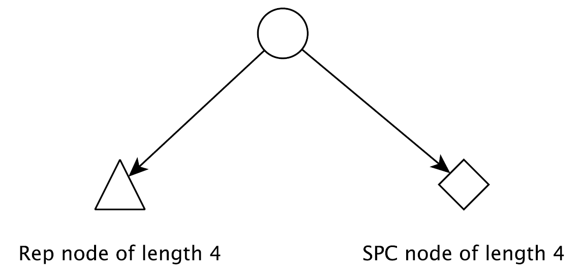
As an example let us consider (8,4) polar code with information set [TeX:] $$\mathcal{I}=\{3,5,6,7\}.$$ The tree of this code consists of two sub-trees: first represents (4,1) repetition code [TeX:] $$\mathcal{R E P}$$ and the second one is (4,3) single parity-check code (4,3). Fig. 3 represents generalized tree of this polar code.
The main idea of GSC/GSCL decoder is to divide a tree of polar code in special nodes listed above and then decode each of these generalized nodes sequentially one by one.
Let us explain the decoding process in more details. Each special node consists of [TeX:] $$n^{\prime}=2^{t}$$ subsequent symbols. During decoding process each node receives [TeX:] $$n^{\prime}$$ input LLR values [TeX:] $$\alpha_{0}^{n^{\prime}-1}$$ and (for GSCL) L or less paths of length [TeX:] $$n^{\prime \prime}$$ with assigned path metrics [TeX:] $$\mathrm{PM}^{l} \text {. }$$ These paths of length [TeX:] $$n^{\prime \prime}$$ are bitsequences that were obtained in previous decoding steps.
After corresponding computations each decoder returns either unique codeword [TeX:] $$\beta_{0}^{n^{\prime}-1} \in\{0,1\}^{n^{\prime}}$$ of subcode corresponed to this special node (for GSC decoding) or a set of at most L binary vectors [TeX:] $$\beta[1], \beta[2], \cdots, \beta\left[L^{\prime}\right]\left(L^{\prime} \leq L\right)$$ of lengths [TeX:] $$n^{\prime}+n^{\prime \prime} \text { with } L^{\prime}$$ smallest values of PM.
Thus after decoding of a given special node we have either decoded bits [TeX:] $$\hat{\mathbf{u}}_{0}^{n^{\prime}+n^{\prime \prime}-1}$$ for GSC, or the list of [TeX:] $$L^{\prime}$$ paths of lengths [TeX:] $$n^{\prime}+n^{\prime \prime} \text { with } L^{\prime}$$ smallest PMs for GSCL.
It should be noted here that path metrics [TeX:] $$\mathrm{PM}^{1}, \cdots, \mathrm{PM}^{L}$$ being calculated for any special node of length [TeX:] $$n^{\prime}$$ are blockwise metrics - it means that they are calculated for the whole codeword of subcode but we can not calculate them for each symbol of subcode.
E. Successive Cancellation Decoding with Flips
The main idea of SC-Flip decoder is to use additional SC decoding attempts in series in the case when an initial SC decoding fails due to a single channel-induced error. During the course of the initial SC decoding, a set of T bit-flipping indices [TeX:] $$\mathcal{F}_{\text {inv }}=\left\{i_{1}, i_{2}, \cdots, i_{T}\right\}$$ (which is also called critical set — CS) are calculated and stored. Indexes in CS are selected in accordance with some criterion (metric). This CS is used when initial SC decoding fails. In this case at most T additional decoding attempts [TeX:] $$S C\left(i_{j}\right), j=1, \cdots, T$$ are applied, where under [TeX:] $$S C\left(i_{j}\right)$$ we denote SC decoding with ijth information bit flipping: i.e., instead of returning bit [TeX:] $$\hat{u}_{i}$$ in accordance with original procedure (2) decoder [TeX:] $$S C\left(i_{j}\right)$$ returns [TeX:] $$1-\hat{u}_{i}.$$
In paper [10] very simple criterion was chosen to construct CS: T indices correspond to T smallest absolute values of output LLRs of initial SC decoding [TeX:] $$\alpha^{(0)}\left[i_{1}\right], \alpha^{(0)}\left[i_{2}\right], \cdots, \alpha^{(0)}\left[i_{T}\right]$$ form a CS. This very simple approach allows to obtain performance of SCL with list size L = 2 for (1024,512) polar code when T = 32.
There are a lot of papers where authors try to improve performance of SCF either by considering more advanced methods for CS construction (for instance making it SNR dependent [13]) or by applying multiple bit-flipping, i.e., flipping more than one bit at each decoding attempt. In paper [18] dynamic SCF decoding (DSCF) was introduce. This decoder in one hand allows multiple flips and in other [TeX:] $$\mathcal{F}_{i n v}$$ is recalculated after each failed decoding attempt. This approach is more powerful and it was shown that DSCF decoding with T = 50 flips has the same performance as SCL-8 and T = 400 flips allow to reach performance of CASCL- 16 for (1024,512) polar code with CRC-16. Multiple bitflipping with nested construction of CS can further improve performance of SC decoding. Nested CS approach was introduced in [17] and simulation results from this paper shows that applying 4-level CS construction jointly with SCF decoding results in approximately the same performance as SCL-32 for (1024,512) polar code with CRC-24. Also it should be noted, that in already mentioned paper [18] multiple flips are also used. For the case of T = 50 2-bit flips are allowed and for T = 400 setting 3-bit flips are allowed. one
The main drawback of SCF decoders based on core SC algorithm is a very strict trade-off between latency and performance. Original SCF decoder from [10] has high latency due to very large number of additional attempts that are required to achieve better performance than SC. At the same time, very simple metric that are used in this decoder can not provide good enough performance that can be comparable with SCL decoders with large list size. More modern algorithms like Dynamic SCF [18] or nested SCF [17] allow to obtain performance of SCL-16 or even SCL-32 but also at the cost of a very high latency due to huge average number of additional SC trials. The most attractive thing here is a space complexity - it remains [TeX:] $$\mathcal{O}(N).$$
F. Successive Cancellation List Decoding with Flips
There is an updated version of flip-based decoder where core SCL with small list size L is used instead of SC. Of course it results in increasing of space complexity from [TeX:] $$\mathcal{O}(N)$$ to [TeX:] $$\mathcal{O}(L N)$$ but number of flips [TeX:] $$\text { (size of } \mathcal{F}_{\text {inv }} \text { ) }$$ can be also reduced significantly. The first paper where SCL decoding with flips (SCLF) was presented is [11]. Authors also provide new method of CS construction. The idea of SCLF is very close to one of SCF. The only difference is that for every additional decoding attempt [TeX:] $$S C L\left(i_{j}\right), j=1, \cdots, T,$$ the SCL decoder chooses L paths of length [TeX:] $$i_{j}$$ with the highest PMs, not the lowest.
In [23] a new metric to construct critical set was proposed. It was shown that core SCL-8 decoder with T = 50 flips outperforms SCL-32 decoder for (256; 128) and (1024,512) polar codes with CRC-9.
Maximal latency of SCLF algorithm is [TeX:] $$\mathcal{O}((T+1) L N \log N)$$ while space complexity is [TeX:] $$\mathcal{O}(L N).$$ But instead of SCF/DSCF decoding SCLF requires significantly smaller number of flips to obtain the reference performance.
The main disadvantage of the decoder in [23] is that the CS metric is symbol-wise: It can not been calculated for some vector of symbols correspond to a subcode of polar code. In our contribution we will discuss how this disadvantage can be overcome.
III. OUR CONTRIBUTION
In this section we give an explanation of our contribution. First, we describe new method of critical set construction for SCLF decoding which can be applied for both symbol-wise traditional decoding and for simplified decoding, based on fast decoding of special nodes. After it we will propose a new generalized SCL decoding with flips (GSCLF) which operates with special patterns of symbols and can achieve significantly better throughput than ordinary SCLF decoder.
A. Differential Critical Set
We propose a new metric which bring in at least the following benefits:
· Suit for both symbol-wise and block-wise SCL decoding
· Low computational complexity
· Better or comparable performance with symbol-wise SCLF
For a SCL decoder, when decoding the ith information bit, at most 2L PMs will be calculated and these PMs will be sorted in an ascending mode. Then the decoder will keep the first half paths with the smaller PMs and discard the second half of the paths with larger PMs. The decoding error probability of i-th information bit is related to the closeness between the value of the PMs in survived paths and the ones in discarded paths. Thus we propose the following metric D to construct CS for symbol-wise decoding:
(3)
[TeX:] $$D[i]=-\min _{l \in \text { Survival }} \mathrm{PM}_{i}^{l}+\min _{l \in \text { Discard }} \mathrm{PM}_{i}^{l}$$T information bits indices with smallest D[i] form the CS:
(4)
[TeX:] $$\operatorname{CS}(T)=\left\{i_{1}, \cdots, i_{T}: D\left[i_{1}\right] \leq \cdots \leq D\left[i_{T}\right]\right\}$$The minimum operation in (3) can be omitted as an ordinary SCL decoding already done the sorting when choosing which paths to be saved.
This differential metric only requires one subtraction operation.
Since the proposed metric depends only on PM from SCL decoding, it can be easily adapted to a GSCL decoder. The only difference is metric calculated on the PMs for subcodes regardless of the exact subcode type. The description how PMs can be calculated for different subcodes type can be found in [24].
It should be mentioned that the proposed differential metric can be considered as simplified version of PM proposed in [12] for [TeX:] $$\alpha=1:$$
(5)
[TeX:] $$E_{i}=\log \frac{\sum_{l=1}^{L} e^{-\mathrm{PM}_{i}^{l}}}{\left(\sum_{l=1}^{L} e^{-\mathrm{PM}_{i}^{L+l}}\right)^{\alpha}}$$Metric (5) can be rewritten as:
Thus D[i] can be stated as the main component of (5) when [TeX:] $$\alpha=1 .$$ As there are no complex calculations, such as [TeX:] $$\log (\cdot)$$ or [TeX:] $$\exp (\cdot),$$ and best exploits the ordinary SCL decoder calculation result and data structure, D[i] is also the extremely simplified metric could preserve all the benefits of (5) stated in [12]. The latest statement comes from the fact that to calculate [TeX:] $$E_{i}$$ one requires to calculate 2L exponential functions of PM, 2L sums of exponents, one calculation of logarithm function and one power function. Thus the complexity [TeX:] $$C_{t o t}$$ for constructing critical set for (N,K) polar codes applying [TeX:] $$E_{i}$$ as follows:
where
1) [TeX:] $$C_{\exp }$$ is a complexity for calculation [TeX:] $$\exp (\cdot)$$
2) [TeX:] $$C_{\log }$$ is a complexity for calculation [TeX:] $$\log (\cdot)$$
3) [TeX:] $$C_{\text {sum }}$$ is a complexity for floating point sum calculation
4) [TeX:] $$C_{\text {pow }}$$ is a complexity for calculation [TeX:] $$x^{\alpha}, x, \alpha \in \mathbb{R}$$
At the same time to calculate D[i] on sorted array of PMs from SCL decoder only one subtraction is required.
Figs. 4–9 illustrate the decoding error distribution versus the index of a critical set, where x-axis represents the index of the critical set based on [TeX:] $$E_{i}$$ metric [12] and differential metric, and the y-asix represents the error probability of the ith bit in received (256, 128 + 16), (512, 256 + 16), (1024, 512 + 16), (1024, 205 + 16), (1024, 648 + 16), (1024, 848 + 16) polar codewords. These results were obtained by decoding of [TeX:] $$10^{6}$$ received codewords for SNR = 2 dB, SNR = 1 dB, SNR = 2.7 dB, and SNR = 3.7 dB in AWGN channel. Simulations obtained for another code constructions (different rates, CRC lenghts and constructions of polar codes) and SNR values show the same behavior.
Here, the code construction is taken from 5G NR standard, the list size of the SCL decoder is 8.
Fig. 4.
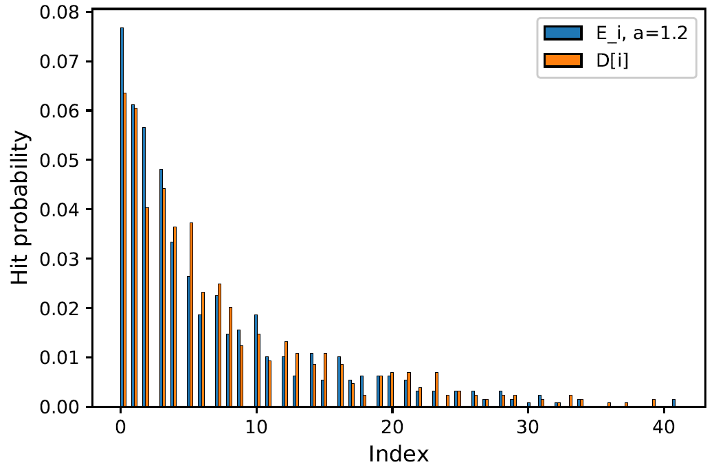
Fig. 5.
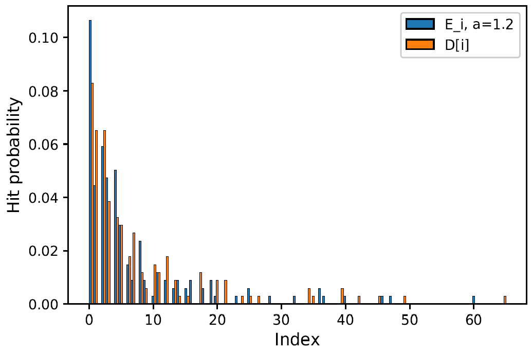
Fig. 6.
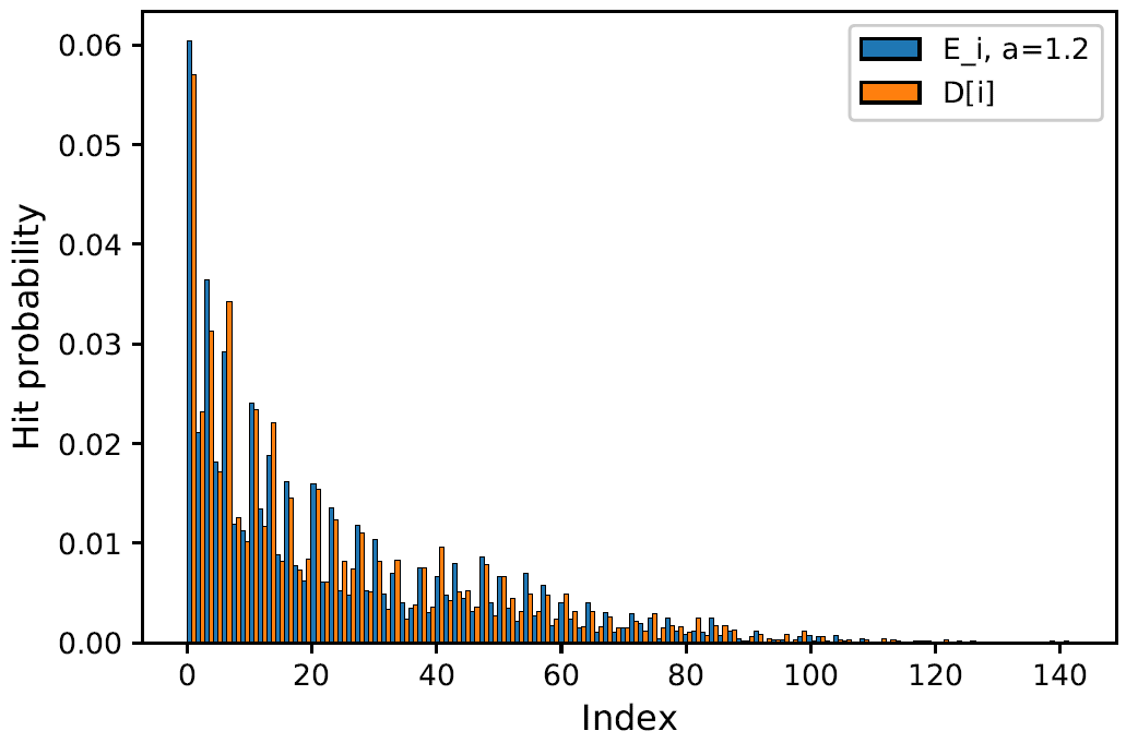
The results show that the error distribution of the differential metric is approximately the same as the distribution of the [TeX:] $$E_{i}$$ metric, which indicates that differential metric requires a the same set size as [TeX:] $$E_{i}$$ metric to cover the first erroneous
Fig. 7.
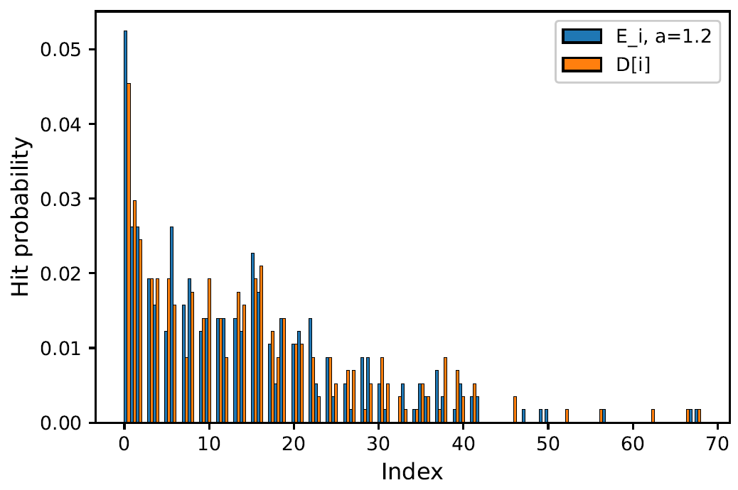
Fig. 8.
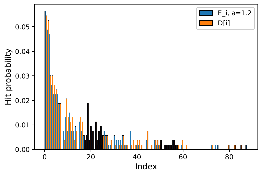
Fig. 9.
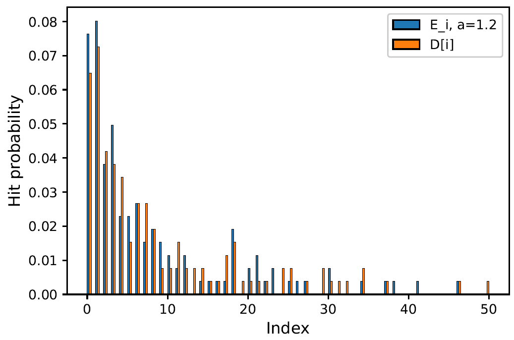
information bit for a fixed probability.
Simulation results provided in Section IV also show that for various code parameters D[i] and [TeX:] $$E_{i}$$ bit-selection metrics used jointly with SCLF decoders have approximately the same error-correction performance. In order to compensate for the biased estimate due to the error propagation the proposed metric D[i] can be straightforwardly generalized in the same manner as [TeX:] $$E_{i}$$. In this case the metric can be calculated as follows:
Now let us show that variation of the parameter α in [TeX:] $$E_{i}$$ does not result in any performance improvement.
Tables I and II presents a simulation results (in terms of FER) for (1024, 512 + 16) 5G NR Polar codes for SCLF decoder with different parameters α. From these tables we can conclude that varying of α does not result in any performance improvement at least for [TeX:] $$F E R \approx 10^{-3}$$ that is working point for applications.
Simulation results we made allow us to conclude that there is no significant improvement in error-correction performance when varying α. Thus instead of using [TeX:] $$D_{\alpha}[i],$$ we will use D[i] further.
B. Subcodes-based Successive Cancellation List Decoding with Flips
In this section we describe how proposed differential metric can be applied for special nodes decoding and flipping in SCLF decoding. Here we propose a new decoder called GSCLF. In fact we show how to modify CS for GSCLF and how to flip the whole special node but single bit. As it was mentioned earlier, the idea of fast list decoding of some special nodes of polar code’s binary tree representation is already known. At the same time there are a several approaches how to organize bit-flipping decoding of polar codes and combine it with SCL decoding. These algorithms are known as SCLF. The main idea of this paper is to combine these two promising approaches for polar codes decoding: Fast list decoding of special nodes that allows to reduce computational complexity and flipping that allows to reduce space complexity of ordinary SCL. To implement this idea we need to characterize each special node in terms of SCL error probability and then flip special nodes where this probability is maximal. Thus the main challenge here is to adapt metrics that are used to construct CS to special nodes.
For simple SCLF decoder with list size L, if ith bit must be flipped, then the flipping is equivalent to choose L paths [TeX:] $$\hat{u}_{0}^{i}[L+1], \cdots, \hat{u}_{0}^{i}[2 L]$$ corresponding to L path metrics with maximal values instead of L paths with minimal ones.
The idea of flipping the whole (instead of symbol flipping) special node s of length [TeX:] $$n^{\prime}=2^{t}$$ and placed in positions from [TeX:] $$i \text { to } i+n^{\prime}-1, i+n^{\prime}-1 \leq N$$ is almost the same: If it is neither trivial nor among first log L non-trivial, then decoder of s — [TeX:] $$\operatorname{Dec}_{\mathbf{s}}\left(\alpha_{i}^{i+n^{\prime}-1},\left(\mathrm{PM}_{1}^{i n}, \cdots, \mathrm{PM}_{L}^{i n}\right)\right) \text { has } n^{\prime} \text { LLR }$$ values and L path metrics [TeX:] $$\mathrm{PM}_{i}^{i n}$$ as an input and produces L surviving paths [TeX:] $$\hat{\mathbf{u}}_{0}^{i+n^{\prime}-1}[1], \cdots, \hat{\mathbf{u}}_{0}^{i+n^{\prime}-1}[L]$$ of length [TeX:] $$n^{\prime}$$ and L corresponding [TeX:] $$\text { PM-s }\left(\mathrm{PM}_{1}^{\text {out }}, \cdots, \mathrm{PM}_{L}^{\text {out }}\right)$$ as output.
If
i.e., at least one of information bits of special node has to be flipped, then output of [TeX:] $$\operatorname{Dec}_{\mathbf{s}}(\cdot, \cdot)$$ changes: Instead of returning L paths with lowest PM, decoder returns L paths [TeX:] $$\hat{\mathbf{u}}_{0}^{i+n^{\top}-1}[L+1], \cdots, \hat{\mathbf{u}}_{0}^{i+n^{\prime}-1}[2 L]$$ with maximal PM-s [TeX:] $$\left(\mathrm{PM}_{L+1}^{\text {out }}, \cdots, \mathrm{PM}_{2 L}^{\text {out }}\right).$$
Such approach of special nodes flipping is sub-optimal for repetition code since each such node extends current list of survival paths twice. In this case flipping of information symbol in repetition code is equivalent to decoding of the corresponded information bit in original SCL decoding—both GSCLF and SCL decoders return the same survival paths for a sequence of bits corresponded to [TeX:] $$\mathcal{R} \mathcal{E} \mathcal{P}.$$
At the same time results of SCL and GSCLF decoders in general differ for [TeX:] $$\mathcal{R}_{1} \text { and } \mathcal{S P} \mathcal{C} \text {. }$$ While SCL decoder makes a decision about new set of survival paths after decoding of each ith information bit (after first [TeX:] $$\log _{2} L$$ information bits), GSCLF decoder updates a set of survival paths after whole subcodes’s decoding. Let us illustrate the main difference between SCL and GSCLF decoders for [TeX:] $$\mathcal{R}_{1}$$ of length [TeX:] $$n^{\prime}=2^{t}, t \in \mathbb{N}.$$ The same idea (with some limitations mentioned below) works also for [TeX:] $$\mathcal{S P C}.$$
[TeX:] $$\mathcal{R}_{1}$$ subcode of length [TeX:] $$n^{\prime}=2^{t}$$ consists of all possible [TeX:] $$N^{\prime}=2^{n^{\prime}}$$ binary sequences [TeX:] $$\mathbf{V}_{1}, \quad \mathbf{V}_{2}, \cdots, \mathbf{V}_{N^{\prime}}$$ of length [TeX:] $$n^{\prime}.$$ Let us assume that this subcode is placed in positions [TeX:] $$i, i+1, \cdots, i+n^{\prime}-1$$ of the whole codeword of polar code. Let us denote by [TeX:] $$\mathrm{y}_{0}^{N-1}$$ a vector of log-likelihoods received from channel. Then the most likely codeword [TeX:] $$\hat{\mathbf{V}}= \left(\hat{v}_{i}, \hat{v}_{i+1}, \cdots, \hat{v}_{i+n^{\prime}-1}\right) \text { of } \mathcal{R}_{1}$$ can be obtained as follows:
(6)
[TeX:] $$\hat{v}_{j}=\left\{\begin{array}{l} 0, \text { if } y_{j}>0 \\ 1, \text { otherwise } \end{array} \quad, j=i, \cdots, i+n^{\prime}-1.\right.$$The second likely codeword [TeX:] $$\tilde{\mathrm{v}} \text { of } \mathcal{R}_{1}$$ can be obtained from [TeX:] $$\hat{\mathbf{v}}$$ by flipping rth bit in [TeX:] $$\hat{\mathbf{V}}$$ that corresponds to smallest absolute LLR value [TeX:] $$\left|y_{r}\right|:$$
Thus GSCLF decoder for [TeX:] $$\mathcal{R}_{1}$$ works as follows: if [TeX:] $$\hat{\mathbf{u}}_{0}^{i-1}[1], \cdots, \hat{\mathbf{u}}_{0}^{i-1}[L]$$ are paths that were survived after decoding of bits from 0 to i-1, then each path [TeX:] $$\hat{\mathbf{u}}_{0}^{i-1}[l], l=1, \cdots, L$$ splits into [TeX:] $$\left(\hat{\mathbf{u}}_{0}^{i-1}[l], \hat{\mathbf{v}}\right) \text { and }\left(\hat{\mathbf{u}}_{0}^{i-1}[l], \widetilde{\mathbf{v}}\right),$$ then PM metric calculates for each of these 2L paths (see [7, eq. (18)]). It means that decoder assigns value [TeX:] $$\text { PM }_{l}^{\text {out }}, l=1, \cdots, 2 L$$ to each path [TeX:] $$\left(\hat{\mathbf{u}}_{0}^{i-1}[l], \hat{\mathbf{v}}\right) \text { and }\left(\hat{\mathbf{u}}_{0}^{i-1}[l], \widetilde{\mathbf{v}}\right)$$ Let us assume that these paths are already sorted by increasing of [TeX:] $$\mathrm{PM}_{l}^{\text {out }}.$$ If
then decoder eliminates paths from L + 1 to 2L with highest path metrics and holds first L paths, else decoder eliminates paths from 1 to L with lowest path metrics and holds last L paths with highest PM.
The idea of [TeX:] $$\mathcal{S P C}$$ list decoding is almost the same. We describe it in few words and highlight the differences between [TeX:] $$\mathcal{S P C} \text { and } \mathcal{R}_{1}$$ list decoders. As in previous example we assume that [TeX:] $$\mathcal{S P C}$$ subcode corresponds to [TeX:] $$i, i+1, \cdots, i+n^{\prime}-1$$ indexes of polar code codeword, [TeX:] $$n^{\prime}=2^{t}.$$
The only difference between [TeX:] $$\mathcal{S P C} \text { and } \mathcal{R}_{1}$$ list decoders is the approach to obtain a set of most likely codewords of the corresponding subcodes. Let us show how most likely
TABLE I
| [TeX:] $$\alpha / S N R$$ | 0 | 0.5 | 1 | 1.5 | 2 |
|---|---|---|---|---|---|
| 1 | [TeX:] $$9.759 \cdot 10^{-1}$$ | [TeX:] $$7.681 \cdot 10^{-1}$$ | [TeX:] $$3.019 \cdot 10^{-1}$$ | [TeX:] $$3.975 \cdot 10^{-2}$$ | [TeX:] $$1.604 \cdot 10^{-3}$$ |
| 1.2 | [TeX:] $$9.760 \cdot 10^{-1}$$ | [TeX:] $$7.690 \cdot 10^{-1}$$ | [TeX:] $$3.014 \cdot 10^{-1}$$ | [TeX:] $$4.031 \cdot 10^{-2}$$ | [TeX:] $$1.622 \cdot 10^{-3}$$ |
| 1.4 | [TeX:] $$9.765 \cdot 10^{-1}$$ | [TeX:] $$7.673 \cdot 10^{-1}$$ | [TeX:] $$3.002 \cdot 10^{-1}$$ | [TeX:] $$3.942 \cdot 10^{-2}$$ | [TeX:] $$1.611 \cdot 10^{-3}$$ |
| 1.6 | [TeX:] $$9.758 \cdot 10^{-1}$$ | [TeX:] $$7.671 \cdot 10^{-1}$$ | [TeX:] $$3.020 \cdot 10^{-1}$$ | [TeX:] $$4.000 \cdot 10^{-2}$$ | [TeX:] $$1.628 \cdot 10^{-3}$$ |
| 1.8 | [TeX:] $$9.767 \cdot 10^{-1}$$ | [TeX:] $$7.687 \cdot 10^{-1}$$ | [TeX:] $$3.005 \cdot 10^{-1}$$ | [TeX:] $$4.008 \cdot 10^{-2}$$ | [TeX:] $$1.613 \cdot 10^{-3}$$ |
| 2 | [TeX:] $$9.778 \cdot 10^{-1}$$ | [TeX:] $$7.700 \cdot 10^{-1}$$ | [TeX:] $$3.027 \cdot 10^{-1}$$ | [TeX:] $$4.034 \cdot 10^{-2}$$ | [TeX:] $$1.630 \cdot 10^{-3}$$ |
TABLE II
| [TeX:] $$\alpha / S N R$$ | 0 | 0.5 | 1 | 1.5 | 2 |
|---|---|---|---|---|---|
| 1 | [TeX:] $$9.621 \cdot 10^{-1}$$ | [TeX:] $$6.887 \cdot 10^{-1}$$ | [TeX:] $$2.152 \cdot 10^{-1}$$ | [TeX:] $$2.051 \cdot 10^{-2}$$ | [TeX:] $$5.640 \cdot 10^{-4}$$ |
| 1.2 | [TeX:] $$9.632 \cdot 10^{-1}$$ | [TeX:] $$6.925 \cdot 10^{-1}$$ | [TeX:] $$2.180 \cdot 10^{-1}$$ | [TeX:] $$2.026 \cdot 10^{-2}$$ | [TeX:] $$5.560 \cdot 10^{-4}$$ |
| 1.4 | [TeX:] $$9.636 \cdot 10^{-1}$$ | [TeX:] $$6.899 \cdot 10^{-1}$$ | [TeX:] $$2.162 \cdot 10^{-1}$$ | [TeX:] $$2.059 \cdot 10^{-2}$$ | [TeX:] $$5.830 \cdot 10^{-4}$$ |
| 1.6 | [TeX:] $$9.619 \cdot 10^{-1}$$ | [TeX:] $$6.905 \cdot 10^{-1}$$ | [TeX:] $$2.172 \cdot 10^{-1}$$ | [TeX:] $$2.079 \cdot 10^{-2}$$ | [TeX:] $$5.680 \cdot 10^{-4}$$ |
| 1.8 | [TeX:] $$9.615 \cdot 10^{-1}$$ | [TeX:] $$6.949 \cdot 10^{-1}$$ | [TeX:] $$2.178 \cdot 10^{-1}$$ | [TeX:] $$2.061 \cdot 10^{-2}$$ | [TeX:] $$6.100 \cdot 10^{-4}$$ |
| 2 | [TeX:] $$9.629 \cdot 10^{-1}$$ | [TeX:] $$6.925 \cdot 10^{-1}$$ | [TeX:] $$2.169 \cdot 10^{-1}$$ | [TeX:] $$2.073 \cdot 10^{-2}$$ | [TeX:] $$5.760 \cdot 10^{-4}$$ |
codewords [TeX:] $$\hat{\mathrm{s}}_{1}, \hat{\mathrm{s}}_{2} \text { of } \mathcal{S P C}$$ can be constructed. The main difference between codewords from [TeX:] $$\mathcal{R}_{1} \text { and } \mathcal{S P C}$$ is that the codewords from the latest must fulfill parity-check constraint. Let us assume that vector [TeX:] $$\mathbf{v}_{i}^{i+n^{\prime}-1}$$ is constructed as in (6). To obtain most likely codeword [TeX:] $$\hat{\mathrm{s}}_{1} \text { of } \mathcal{S} \mathcal{P} \mathcal{C}$$ one apply the following algorithm:
1) Set [TeX:] $$v_{i}=0$$ since first symbol of [TeX:] $$\mathcal{S P C}$$ is frozen
2) Calculate [TeX:] $$q=\bigoplus_{j=i+1}^{i+n^{\prime}-1} v_{j},$$ where [TeX:] $$\oplus$$ means modulo-2 sum.
3) If q = 0 then set [TeX:] $$\hat{\mathrm{s}}_{1}=\mathrm{v}$$ and terminate.
4) If q = 1 then find index r of least reliable bit among [TeX:] $$i+1, \cdots, i+n^{\prime}-1$$ bits
5) Update [TeX:] $$v_{r}=1-v_{r}.$$
6) Set [TeX:] $$\hat{\mathrm{s}}_{1}=\mathrm{v}$$ and terminate
The second most likely codeword [TeX:] $$\hat{\mathbf{s}}_{2}$$ can be obtained from [TeX:] $$\hat{\mathbf{s}}_{1}$$ by flipping two least reliable bits of [TeX:] $$\hat{\mathrm{s}}_{1}.$$
All other steps of [TeX:] $$\mathcal{S P C}$$ list decoding and flipping are the same as for [TeX:] $$\mathcal{R}_{1}.$$
It should be noted that subcodes’ flipping approach does not take into account two facts that are rather important in original SCLF:
1) Number of information bits be flipped in subcode
2) Positions of these bits
It means that proposed rule of subcodes flipping can significantly reduce number of flips in CS. It doesn’t make sense to make T more than number of non-trivial (not [TeX:] $$\left.\mathcal{R}_{0}\right)$$ subcodes of polar code. The further increasing of T does not result in any performance improvement in this scheme.
The subcodes structure of 5G NR polar codes with CRC-16 and code rate R = 0.5 are listed in Table III.
It can be noted from Table III that for short polar codes number of non-trivial special nodes is very limited. If number of accepted flips T exceeds number of non-trivial special nodes then further simplifications of GSCLF are possible: In this case we can eliminate “on-line” CS construction, calculate it offline and use as an external parameter of GSCLF.
Summarizing all written above we can give an algorithmic description of proposed decoder.
Algorithm
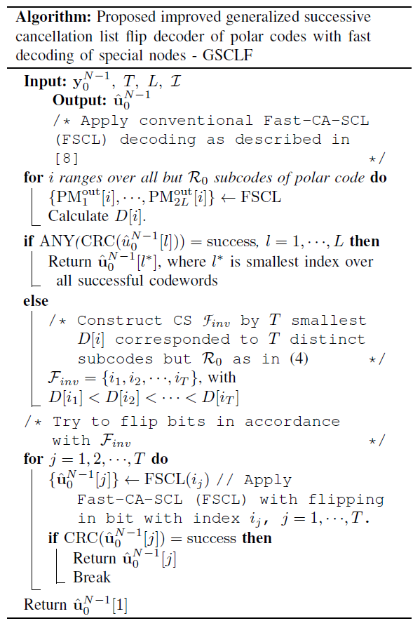
TABLE III
| Polar code | [TeX:] $$\mathcal{R}_{1}$$ | [TeX:] $$\overline{\mathcal{R E P}}$$ | [TeX:] $$\mathcal{S P C}$$ | Max. T |
|---|---|---|---|---|
| (64, 32+16) | 6 | 3 | 1 | 10 |
| (128, 64+16) | 6 | 7 | 5 | 18 |
| (256, 128+16) | 6 | 9 | 9 | 24 |
| (512, 256+16) | 11 | 17 | 13 | 41 |
| (1024, 512+16) | 17 | 26 | 26 | 69 |
IV. SIMULATION RESULTS
A. Simulation Results — Performance Analysis
In this section, we compare the frame error rate (FER) performance of the proposed SCLF/GSCLF decoders based on our proposed critical set construction. We implement two versions of SCLF - symbol-wise (called SCLF Diff, T = x) and generalized subcodes-based GSCLF versions (called GSCLF, T = x). We compare our proposed schemes with SCLF decoder based on CS constructed as described in [12] (called further CA-SCL-1, T = x). The 16-bit CRC with the generator polynomial [TeX:] $$g(x)=x^{16}+x^{15}+x^{2}+1$$ is used for codeword selection in all decoding schemes (SCLF, GSCLF, CA-SCL) that are used for performance comparison). This CRC is combined with half-rate 5G NR polar codes with lengths N = 1024, 512, 256, and (1024, 648). We also consider (1024, 205) and (1024, 848) 5G NR polar codes which have exactly 50 different subcodes but [TeX:] $$\mathcal{R}_{0}.$$ It means that for T = 50 all information symbols (grouped by special nodes) will be flipped.
It must be stated here that for comparison we use only PM proposed in [12] but not the whole decoding scheme since it has significantly higher complexity due to recalculation of CS after each unsuccessful decoding attempt and multilevel flips in [12]. We will denote SCLF decoder with CS based on [12] by CA-SCL-1. As in [12] we use [TeX:] $$\alpha=1.2$$ for [TeX:] $$E_{i}$$ calculation.
AWGN channel and binary phase shift keying (BPSK) are used for simulation.
We consider two setups: When number of flips is small (T = 10) and when it is significantly large (T = 50). For symbol-wise decoders maximal possible number of flips is limited by the number of information symbols of code but for generalized decoder it is reasonable to limit this value by the number of non-trivial subcodes [TeX:] $$\mathcal{R}_{1}, \mathcal{R} \mathcal{E} \mathcal{P}, \mathcal{S P C}.$$ (256, 128+ 16) and (512, 256+16) codes have less than 50 such subcodes and thus for this case we limit number of flips for subcodes based decoders by 10.
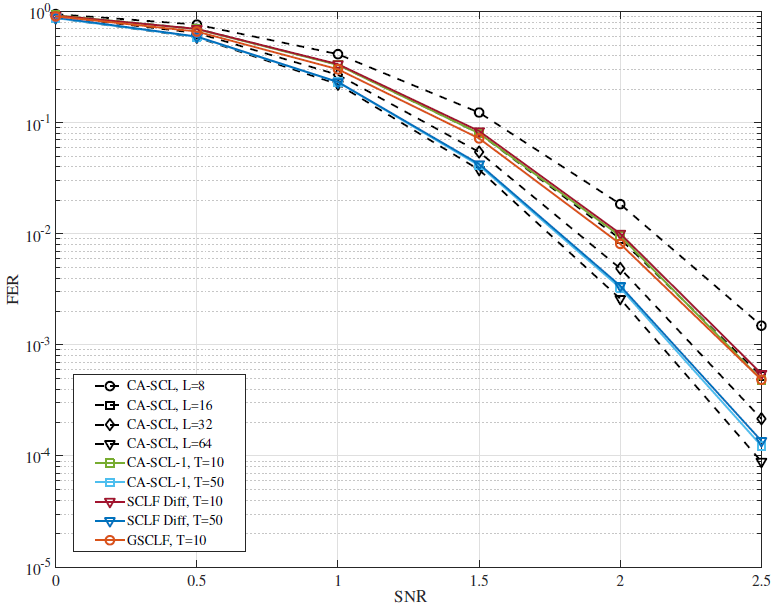
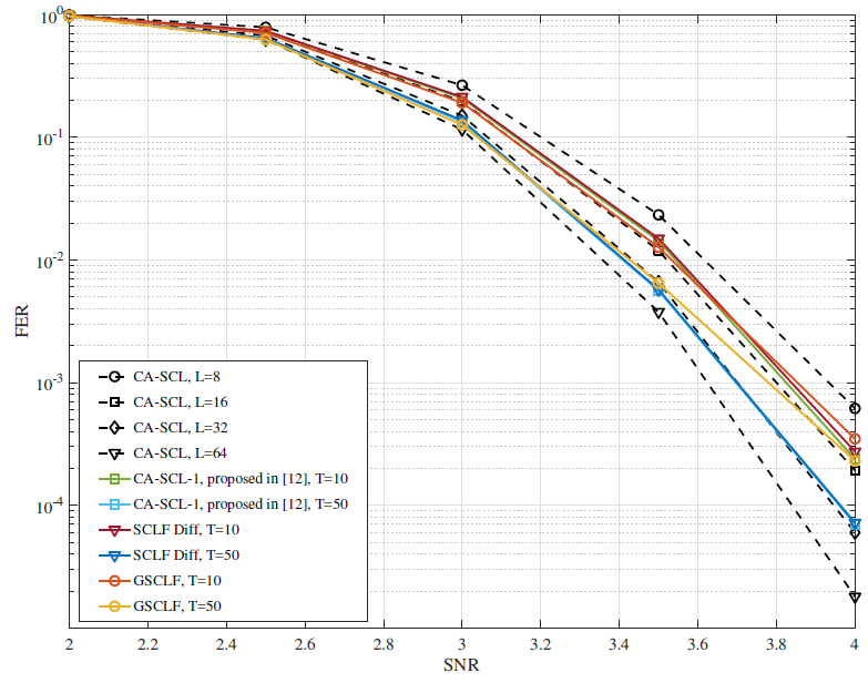
Figs. 10–13 represents simulation results for the proposed decoders with our new metric in comparison with scheme from [12]. As it can be noticed new SCLF / GSCLF decoders have the same performance as more complex ones from [12] both for T = 10 and T = 50. For (256, 128 + 16) GSCLF with T = 10 even has slightly better performance than bit-wise schemes.
As it can be seen from Figs. 10–13 for moderate length polar codes [TeX:] $$(N \leq 512)$$ decoders based on bit-flipping with T = 50 can achieve the performance of SCL-64 decoder. For polar codes of length N = 1024 flipping schemes (including CA-SCL-1 with [TeX:] $$\alpha=1.2)$$ with T = 50 can achieve the
Fig. 10.
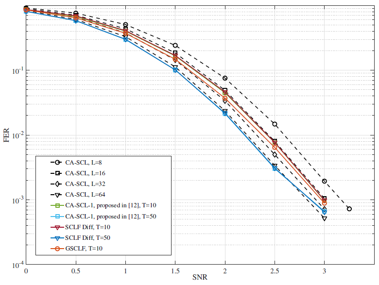
Fig. 11.
performance of CA-SCL, L = 32 only. However, in [12] (Fig. 9) it was shown that CA-SCL-1 with T = 50 and [TeX:] $$\alpha=1.2$$ can achieve the performance of CA-SCL L = 64 for (1024; 512 + 16) polar code. This discrepancy in the simulation results can be explained as follows: it is known that performance of different decoding schemes depend on structure of polar code. In our simulations we use 5G NR polar code. Article [12] does not indicate the structure of the used polar codes. Perhaps, for other constructions of polar codes, the simulation results will be different, but for fair comparison we choose the decoder parameters [TeX:] $$(\mathrm{CRC}, L, \alpha, T)$$ coincide with ones in [12].
Now let us present the behavior of bit-flipping and GSCLF decoders based on [TeX:] $$E_{i}$$ and D[i] metrics for high-rate codes. We compare the performance of CA-SCL-16, CA-SCL-32, CA-SCL-64, bit-flipping decoders based on [TeX:] $$E_{i}$$ and D[i], and
Fig. 12.
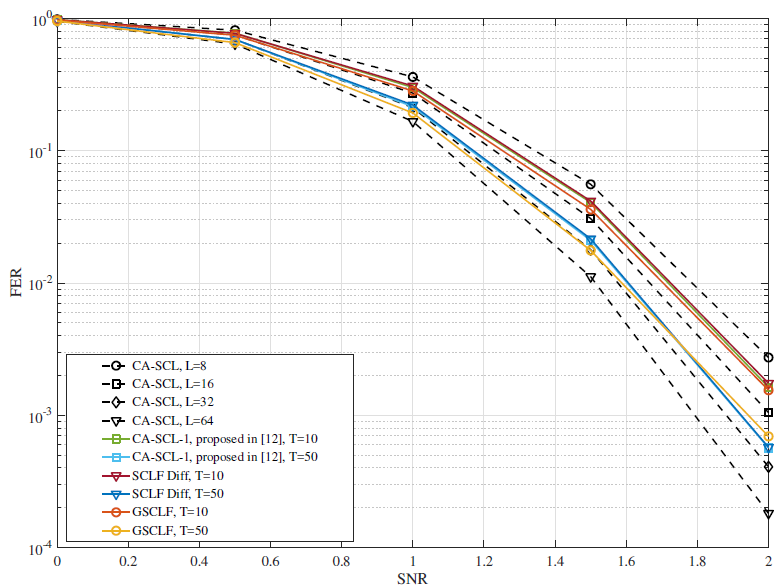
Fig. 13.
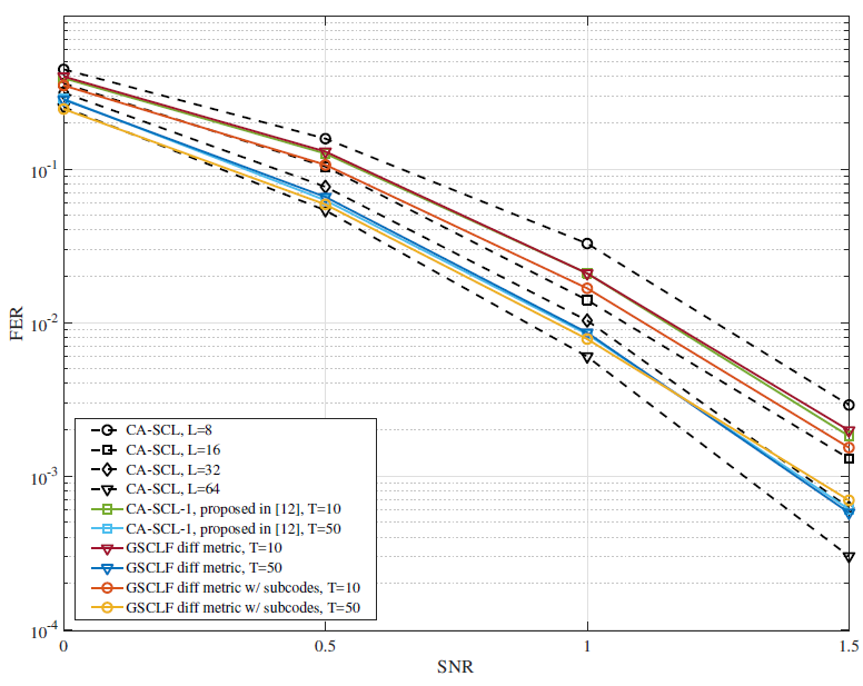
GSCLF decoders based on D[i]. We choose (1024, 648+16) and (1024, 848 + 16) polar codes. The latest code has 50 different non-trivial subcodes as (1024, 205 + 16) code.
From Fig. 14 we can conclude that while bit-flipping decoders based on [TeX:] $$E_{i}$$ and D[i] metrics have identical performance that coincides (for T = 50) with CA-SCL, L = 32 decoder, GSCLF decoder shows worse performance than symbol-wise decoders. This fact can be explained as follows: the higher rate of polar code, the more number of [TeX:] $$\mathcal{S P C}$$ and [TeX:] $$\mathcal{R}_{1}$$ codes in it’s decoding tree. Since these code have high rate, then its’ list decoding without tree traversal described in Section II-D provides significantly worse performance than SCL decoding, and the longer [TeX:] $$\mathcal{S P C} \text { or } \mathcal{R}_{1}$$ code, the higher difference between SCL and direct list decoding without tree traversal.
Finally, let us present simulation results for 5G NR
Fig. 14.
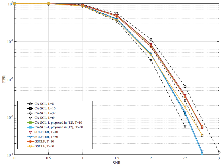
Fig. 15.
(1024, 848 + 16) polar code.
Simulation results presented in Fig. 15 proofs the hypothesis that the higher code rate the worse performance of GSCLF decoder, when the number of flips T is fixed. Since (1024, 848 + 16) polar code has more longer [TeX:] $$\mathcal{S P C} \text { and } \mathcal{R}_{1}$$ codes than (1024, 648 + 16) and especially (1024, 512 + 16) code, then GSCLF decoder results in the worst performance. We suppose that this behavior is common for all simplified (fast) SCL decoders since the structure of high-rate polar codes involves a lot of long [TeX:] $$\mathcal{S P C} \text { and } \mathcal{R}_{1}$$ codes, where simplified list decoding operates only with a very limited number of codeword-candidates. This fact was already mentioned in [24] where authors found error-correction performance loss when length of [TeX:] $$\mathcal{S P C}$$ code is higher than 8. One possible way to overcome this issue is to divide long [TeX:] $$\mathcal{S P C}$$ code on shorter subcodes and decode them separately. At the same time this
Fig. 16.
approach results in complexity increasing and we will not implement it in this paper.
Thus the best use cases for proposed GSCLF decoder are such applications where either low-rate or short length polar codes are exploited.
B. Simulation Results — Complexity Analysis
As it was mentioned above, high rate polar codes are not use cases of the proposed GSCLF decoder with fast special nodes decoding. Thus we present a complexity analysis of GSCLF decoder for codes with moderate and low code rates, for whom GSCLF decoder is more applicable.
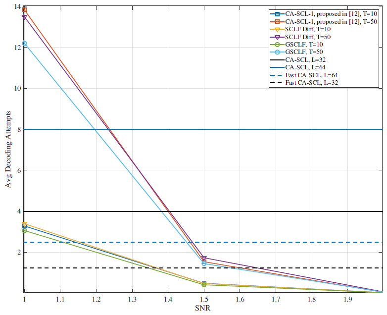
Before we present a detailed complexity analysis let us show the dependence between average number of additional decoding attempts (flips) and SNR for (1024, 512) polar code with CRC-16 for different decoding algorithms with flips. This value is normalized by the complexity of CA-SCL decoding with L = 8. We also add complexities of CASCL with L = 32 and L = 64 (horizontal solid lines) and complexities of their fast simplified versions proposed in [8] (dashed horizontal lines).
Fig. 16 shows the average number of additional decoding attempts for every decoding scheme which is normalized by the complexity of CA-SCL decoding with L = 8. It can be also noticed that the proposed schemes have either the same number of additional flips or even smaller for subcodes based decoders. But it will be shown that regardless of the fact that the number of attempts is about the same for already known and proposed decoding schemes, GSCLF algorithm has significantly lower computational complexity. Comparing our proposed decoders with CA-SCL or fast CA-SCL proposed in [8] we can conclude that all bit-flipping schemes lose in complexity to CA-SCL and fast CA-SCL decoders in low SNR regions. At the same time average number of decoding attempts drops rapidly as the SNR increases, and proposed decoders have lower complexity compared to CA-SCL and Fast CA-SCL decoding with L = 32 and 64 in the mediumto- high SNR region.
Now let us present the detailed complexity analysis (in terms of average number of different operations) of the proposed decoders and compare them with CA-SCL-16, CA-SCL-32, fast CA-SCL decoders, proposed in [8], and stack decoder (SCS) from [25]. For all implementations of SCL decoders we use simplified LLR-based versions of them, where logarithmic and exponential calculations are omitted [26]. The results are collected not for one decoding iteration (one decoding attempt in flipping scheme) but for the full decoding scheme averaged by [TeX:] $$10^{6}$$ decoding attempts for fixed SNR = 2. All values in the table are counted in thousands [TeX:] $$(\times 1000).$$ For all considered decoding schemes we count numbers of different operations that are used in decoding. It means that when any decoder applies some calculation, like D[i] evaluation for ith symbol, we suppose that decoder uses one [TeX:] $$\cdot(-1)$$ operation and one sum operation, assuming that [TeX:] $$P M_{i}^{1} \text { and } P M_{i}^{L+1}$$ are already calculated in previous decoding steps. We first calculate the total number of each operation mentioned in tables, and then divide these amounts on total trials of decodings.
In considered schemes of CA-SCL-1 proposed in [12], SCLF Diff, GSCLF we assume that the core SCL decoder has list size L = 8. All polar codes use CRC-16 for errors detection.
Now let us describe headers of tables. Tables IV–VII have 9 columns:
1) Algorithm:
· CA-SCL-L — is a ordinary CRC-aided SCL with list size L
· Fast CA-SCL-L — improved CA-SCL-L decoder with fast decoding of special nodes [8]
· CA-SCL-1, T = x — is a decoder with metric proposed in [12] with x additional decoding attempts
· SCLF Diff, T = x — is a symbol-wise decoder with new proposed metric and with x additional decoding attempts
· GSCLF, T = x — is a subcodes-based decoder with new proposed metric and with x additional decoding attempts
· SCS, L = x, D = y — Successive Cancellation Stack decoder with list L and size of stack D
2) # sums — number of floating point additions
3) # mults — number of floating point multiplications
4) # comps — number of comparing numbers: [TeX:] $$>, <, =, \leq, \geq$$
5) # [TeX:] $$\exp (\cdot)-$$ number of exponents calculations [TeX:] $$\exp (\cdot)$$ (used only in a metric (5) calculation in CA-SCL-1)
6) # [TeX:] $$\log (\cdot)-$$ number of logarithms calculations [TeX:] $$\log (\cdot)$$ (used only in a metric (5) calculation in CA-SCL-1)
7) # [TeX:] $$\oplus-$$ number of modulo-2 XORs
8) # [TeX:] $$\cdot(-1)-$$ number of inversions (multiplications on -1). Excluded from “number of muls”
9) total — Total number of operations
From Tables IV–VII and the previously obtained simulation results, we can conclude that although the proposed metric D[i] applied for symbol-by-symbol decoding does not provide
TABLE IV
| Algorithm | # sums | # mults | # comps | [TeX:] $$\# \exp (\cdot)$$ | [TeX:] $$\# \log (\cdot)$$ | [TeX:] $$\# \oplus$$ | [TeX:] $$\# \cdot(-1)$$ | Total |
|---|---|---|---|---|---|---|---|---|
| CA-SCL-16 | 229.99 | 52.22 | 124.37 | 0 | 0 | 26.61 | 9.91 | 443.10 |
| Fast-CA-SCL-16 | 201.89 | 12.3 | 160.37 | 0 | 0 | 23.20 | 2.34 | 400.03 |
| CA-SCL-32 | 473.13 | 101.86 | 253.90 | 0 | 0 | 52.27 | 19.49 | 900.65 |
| Fast-CA-SCL-32 | 399.71 | 24.20 | 312.93 | 0 | 0 | 45.83 | 4.58 | 787.25 |
| CA-SCL-1, T=10 | 188.91 | 48.97 | 103.93 | 4.55 | 2.58 | 21.03 | 14.60 | 384.57 |
| SCLF, Diff, T=10 | 186.67 | 49.44 | 106.3 | 0 | 0 | 21.29 | 13.92 | 377.62 |
| GSCLF, Diff, T=10 | 154.25 | 9.50 | 127.00 | 0 | 0 | 17.5 | 1.77 | 310.02 |
| CA-SCL-1, T=50 | 300.58 | 78.88 | 165.18 | 6.37 | 4.90 | 33.94 | 22.86 | 612.71 |
| SCLF, Diff, T=50 | 297.82 | 79.21 | 167.27 | 0 | 0 | 34.14 | 22.15 | 600.59 |
| SCS, L=32, D=L*N | 43.38 | 2.31 | 8438.69 | 0 | 0 | 1.03 | 4.37 | 8489.78 |
TABLE V
| Algorithm | # sums | # mults | # comps | [TeX:] $$\# \exp (\cdot)$$ | [TeX:] $$\# \log (\cdot)$$ | [TeX:] $$\# \oplus$$ | [TeX:] $$\# \cdot(-1)$$ | Total |
|---|---|---|---|---|---|---|---|---|
| CA-SCL-16 | 469.82 | 03.54 | 266.16 | 0 | 0 | 59.77 | 19.53 | 918.82 |
| Fast-CA-SCL-16 | 378.62 | 23.28 | 314.49 | 0 | 0 | 49.29 | 4.33 | 770.01 |
| CA-SCL-32 | 975.37 | 202.60 | 546.18 | 0 | 0 | 117.61 | 38.48 | 1880.21 |
| Fast-CA-SCL-32 | 753.59 | 45.95 | 614.53 | 0 | 0 | 97.91 | 8.59 | 1520.57 |
| CA-SCL-1, T=10 | 283.00 | 70.66 | 162.77 | 7.36 | 3.86 | 34.56 | 21.25 | 583.46 |
| SCLF, Diff, T=10 | 277.80 | 71.28 | 166.88 | 0 | 0 | 34.99 | 19.88 | 570.83 |
| GSCLF, Diff, T=10 | 216.59 | 13.33 | 186.71 | 0 | 0 | 27.86 | 2.46 | 446.95 |
| CA-SCL-1, T=50 | 332.71 | 83.63 | 191.39 | 8.41 | 5.64 | 40.94 | 24.78 | 687.50 |
| SCLF, Diff, T=50 | 331.12 | 82.19 | 197.57 | 0 | 0 | 41.84 | 23.66 | 677.82 |
| SCS, L=32, D=L*N | 134.59 | 5.11 | 33696.20 | 0 | 0 | 2.30 | 9.45 | 33847.65 |
TABLE VI
| Algorithm | # sums | # mults | # comps | [TeX:] $$\# \exp (\cdot)$$ | [TeX:] $$\# \log (\cdot)$$ | [TeX:] $$\# \oplus$$ | [TeX:] $$\# \cdot(-1)$$ | Total |
|---|---|---|---|---|---|---|---|---|
| CA-SCL-16 | 969.86 | 209.39 | 573.54 | 0 | 0 | 134.55 | 39.26 | 1926.60 |
| Fast-CA-SCL-16 | 789.09 | 43.33 | 679.29 | 0 | 0 | 108.67 | 8.49 | 1628.87 |
| CA-SCL-32 | 2023.57 | 409.94 | 1177.65 | 0 | 0 | 264.60 | 77.44 | 3953.20 |
| Fast-CA-SCL-32 | 1563.29 | 85.47 | 1319.63 | 0 | 0 | 215.60 | 16.84 | 3200.83 |
| CA-SCL-1, T=10 | 533.18 | 129.49 | 319.19 | 10.34 | 6.93 | 70.94 | 38.72 | 1108.79 |
| SCLF, Diff, T=10 | 517.06 | 129.14 | 323.80 | 0 | 0 | 71.04 | 35.62 | 1076.66 |
| GSCLF, Diff, T=10 | 416.63 | 22.73 | 368.58 | 0 | 0 | 56.61 | 4.40 | 868.95 |
| CA-SCL-1, T=50 | 538.73 | 134.28 | 330.51 | 10.60 | 7.38 | 73.59 | 40.01 | 1135.10 |
| SCLF, Diff, T=50 | 522.04 | 134.63 | 336.80 | 0 | 0 | 74.07 | 37.09 | 1104.63 |
| GSCLF, Diff, T=50 | 434.22 | 23.70 | 384.06 | 0 | 0 | 59.03 | 4.59 | 905.60 |
| SCS, L=32, D=L*N | 454.10 | 11.26 | 134686 | 0 | 0 | 5.12 | 19.09 | 135175.57 |
TABLE VII
| Algorithm | # sums | # mults | # comps | [TeX:] $$\# \exp (\cdot)$$ | [TeX:] $$\# \log (\cdot)$$ | [TeX:] $$\# \oplus$$ | [TeX:] $$\# \cdot(-1)$$ | Total |
|---|---|---|---|---|---|---|---|---|
| CA-SCL-16 | 615.61 | 146.40 | 380.98 | 0 | 0 | 104.44 | 25.21 | 1272.64 |
| Fast-CA-SCL-16 | 436.94 | 24.52 | 390.29 | 0 | 0 | 75.41 | 3.47 | 930.63 |
| CA-SCL-32 | 1202.40 | 274.74 | 737.70 | 0 | 0 | 197.80 | 47.93 | 2460.57 |
| Fast-CA-SCL-32 | 853.07 | 47.50 | 741.43 | 0 | 0 | 146.67 | 8.86 | 1797.53 |
| CA-SCL-1, T=10 | 338.84 | 86.70 | 211.07 | 7.12 | 5.07 | 55.83 | 20.83 | 725.46 |
| SCLF, Diff, T=10 | 332.10 | 86.55 | 212.96 | 0 | 0 | 55.87 | 19.54 | 707.02 |
| GSCLF, Diff, T=10 | 228.72 | 12.59 | 214.86 | 0 | 0 | 38.63 | 1.78 | 496.58 |
| CA-SCL-1, T=50 | 339.54 | 86.88 | 211.51 | 7.55 | 5.17 | 55.95 | 20.87 | 727.47 |
| SCLF, Diff, T=50 | 332.24 | 86.58 | 213.05 | 0 | 0 | 55.89 | 19.55 | 707.31 |
| GSCLF, Diff, T=50 | 228.97 | 12.60 | 215.10 | 0 | 0 | 38.67 | 1.78 | 497.12 |
a significant reduction in complexity, nevertheless, the GSCLF decoder with this metric can significantly reduce the number of operations required for decoding a polar code. Although the GSCLF decoder uses a slightly larger number of comparison operations than bit flipping decoders, it can significantly reduce the number of such complex operations as multiplications in comparison not only with CA-SCL-16 and especially CASCL- 32 decoders and their fast modifications [8] but also with CA-SCL-1 with metric proposed in [12] and with bit flipping decoder SCLF with D[i] metric. Let us also remind that space complexity of GSCLF decoder is [TeX:] $$\mathcal{O}(L N),$$ where L is list size of the core decoder. For flipping decoders presented in Tables IV–VII, L = 8. Thus for practical important FER values (from 0.05 to [TeX:] $$10^{-4}$$ at SNR = 2 for different polar codes) new proposed GSCLF decoder reduces number of operations from 66% to 80% for different parameters of polar codes and different number of flips while requiring approximately 4 times smaller memory than CA-SCL-32 decoder.
We emphasize again that the most significant complexity reduction is achieved on the most computationally complex operations. It is a main reason why further complexity comparisons between decoding algorithms will be divided into two groups: first we compare decoders taking into account total number of operations except multiplications, exp() and log() and second we compare decoders in terms of number of the most expensive operations — multiplications, exp() and log().
In the last three rows of the table we present complexity estimations for different polar codes decoded by succesive cancellation stack decoder (SCS) with list size L = 32 and stack size D = LN, where N is a code length. In accordance with [25] these parameters of SCS allow to obtain performance of SCL-32 decoder. As it can be found from the Tables IV–VI, SCS can significantly reduce number of nearly all operations applied during decoding in comparison not only with CASCL- 32 but also with GSCLF. At the same time a number of comparison operations in SCS increases dramatically with code length even in comparison with CA-SCL-32. Although, of course, it should be noted that comparison operations are much simpler than operations such as multiplication, calculating logarithms, etc. In addition, main drawback of the SCS decoder should be noted. The memory consumption of SCS can be estimated as [TeX:] $$\mathcal{O}(D N)$$ which is significantly larger than [TeX:] $$\mathcal{O}(D N)$$ for CA-SCL-L decoder. Thus the proposed GSCLF decoder might be considered as a competitor to SCS especially in applications and devices that imply significant memory limitations.
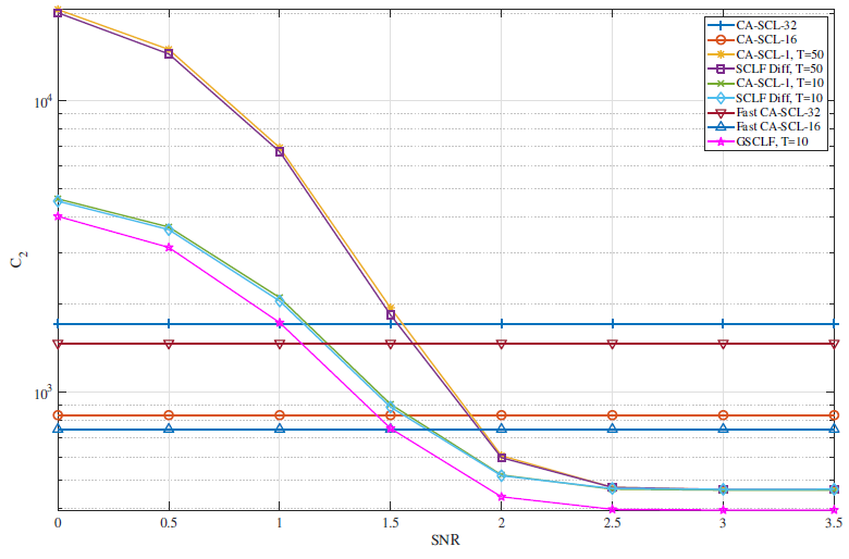
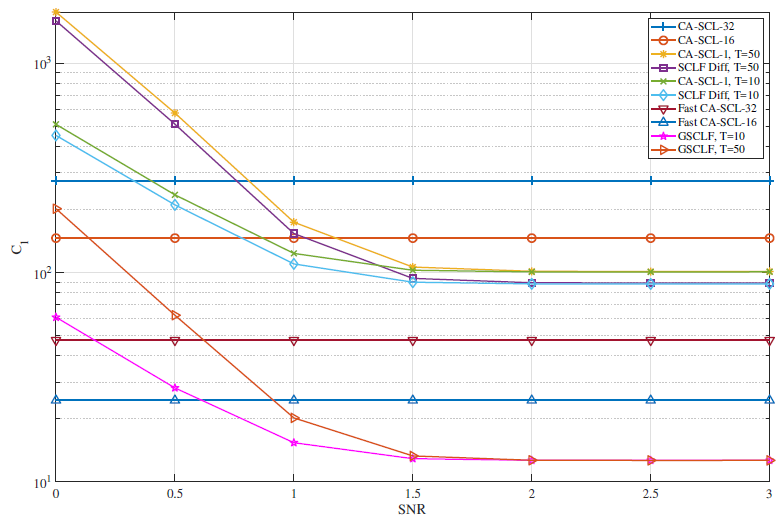
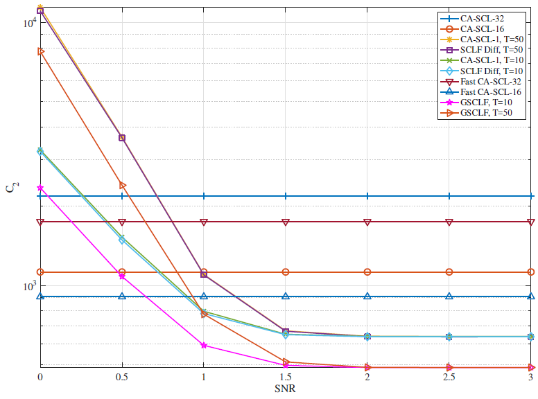
Let us present a graphical representation of the dependence between code construction and complexities [TeX:] $$C_{1}=\# \text { mults }+ \# \exp (\cdot)+\# \log (\cdot) \text { and } C_{2}=\text { total }-C_{1}$$ of different decoding algorithms represented in Tables IV–VII.
Figs. 17–20 demonstrate that for all parameters of polar codes GSCLF decoder with either T = 10 or T = 50 provide the lowest computational complexity in comparison with both SCL/Fast-SCL with larger list size and with SCLF decoder with the same list size and T as in GSCLF but with symbol-by-symbol calculations: Average reduction in complexity due to subcodes decoding is 23% for T = 10 and T = 50. More significant difference is achieved on low-
Fig. 17.
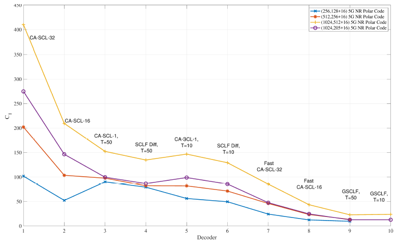
Fig. 18.
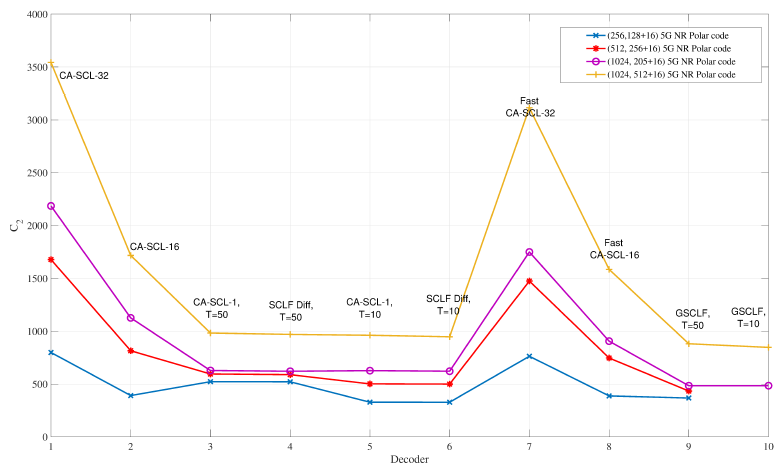
Fig. 19.
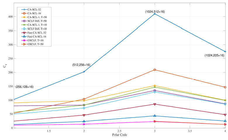
rate codes: for (1024, 205 + 16) code the difference in the number of operations between the SCLF and GSCLF decoder is 32% for T = 10. It should be noted that GSCLF decoders provide the most significant complexity reduction in terms of multiplications [TeX:] $$\left(C_{1}\right.$$ complexity), while [TeX:] $$C_{2}$$ complexity of GSCLF is approximately the same as for bit-flipping decoders with the same T value.
Fig. 20.
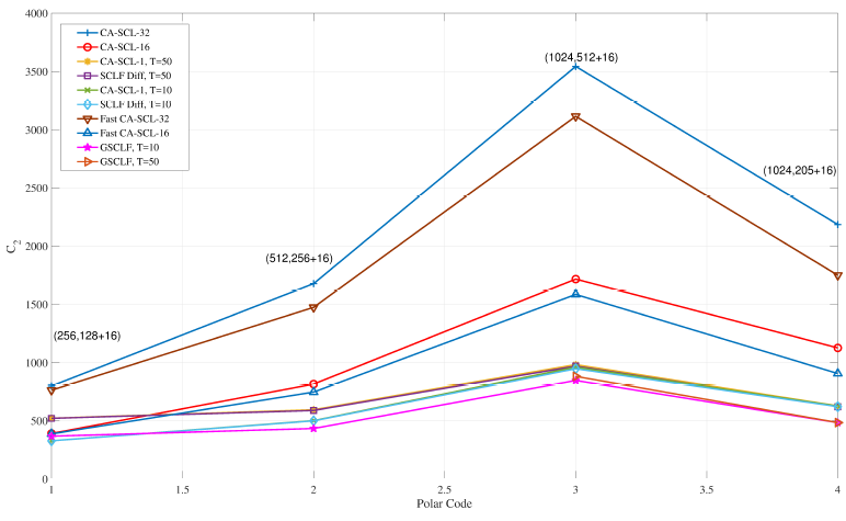
Fig. 21.
Also it can be noticed that curves in Figs. 17–20 corresponded to either GSCLF decoder with T = 50 or polar codes of length N = 256 and N = 512 have less points than other curves. This comes from the fact that polar codes with N = 256 and N = 512 are not decoded by GSCLF decoder with T = 50 since these codes have less than 50 non-trivial subcodes.
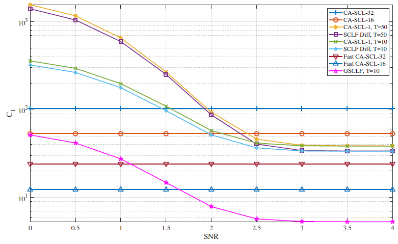
Finally, we present a simulation results of the dependence of the total decoding complexity for different SNR ratio for various decoders and various parameters of polar codes.
Simulation results presented in Figs. 21–28 demonstrate that for practically significant signal-to-noise ratios (corresponding to the error probability per block less than 0.01), the proposed GSCLF decoders based D[i] metric with a list size L = 8 provide a significant reduction in computational complexity compared to SCL-16 and SCL-32, and at sufficiently high signal-to-noise ratios (corresponding to the error probability per block less than 0.001) are less complex than fast simplified versions of SCL-16 and SCL-32 [8]. In addition, for all signalto- noise ratios, GSCLF decoders have complexity less than bitwise SCLF decoders with D[i] CS construction and CA-SCL-1 with metric from [10]. Moreover, previously it was shown that GSCLF decoders have significantly lower [TeX:] $$C_{1}$$ complexity (complexity in terms of multiplications, [TeX:] $$\log (\cdot), \exp (\cdot))$$ than
Fig. 22.
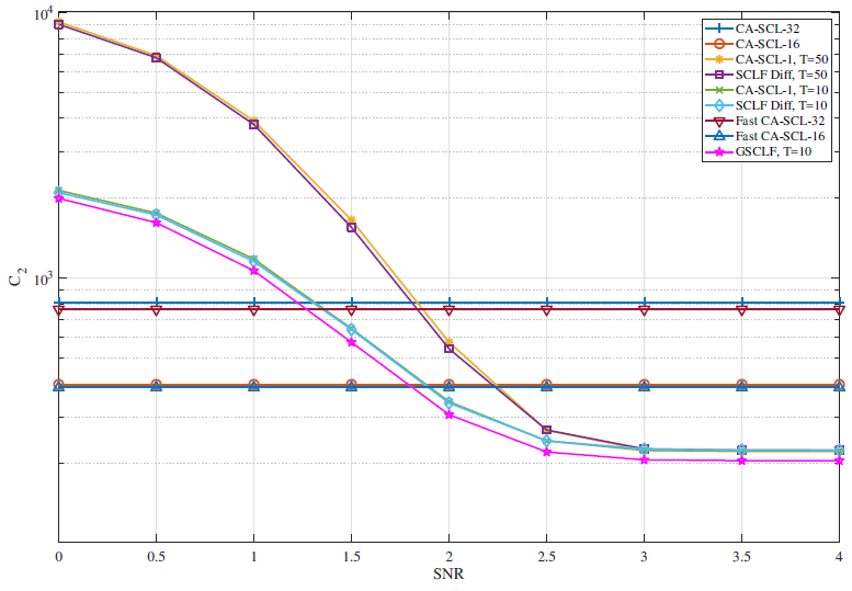
Fig. 23.
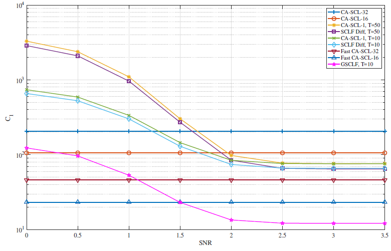
Fig. 24.
other competitors for different polar codes and SNR = 2 dB. Simulation results provided in Figs. 21–28 show that GSCLF decoder has significantly lower [TeX:] $$C_{1}$$ complexity than bit-flipping decoders for wide range of SNR and approximately the same [TeX:] $$C_{2}$$ complexity. Comparing the complexity of GSCLF and fast
Fig. 25.
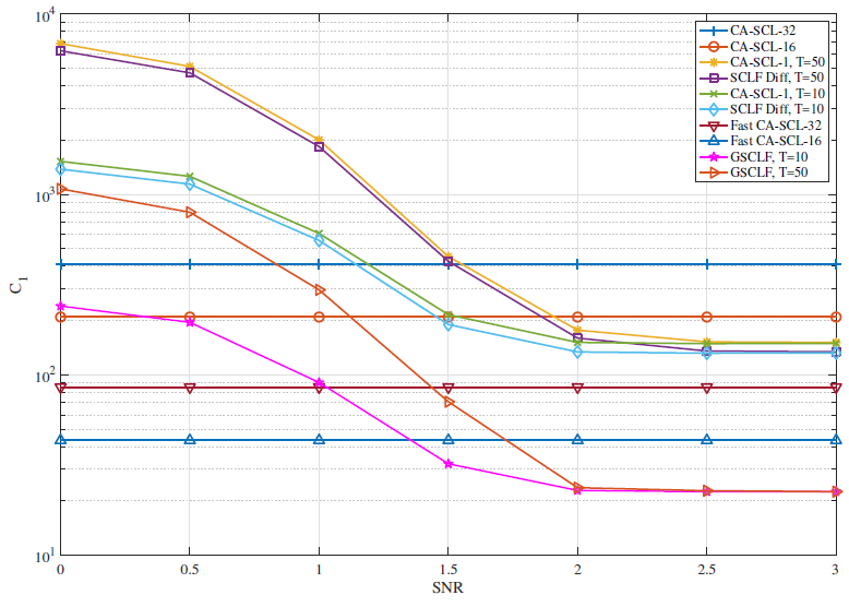
Fig. 26.
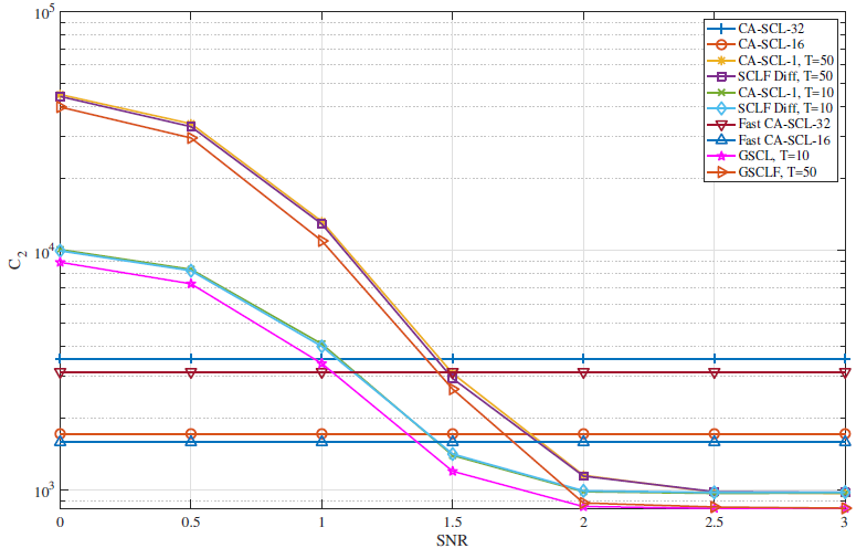
Fig. 27.
CA-SCL decoders [8], we can conclude that GSCLF also provides both [TeX:] $$C_{1} \text { and } C_{2}$$ complexities reduction for SNR values correspond to practical FER values [TeX:] $$(\leq 0.01).$$
Thus, the use of GSCLF is justified at sufficiently high
Fig. 28.
signal-to-noise ratios, where they have a complexity that is less than that of list decoders, and, in addition, this class of decoders should always be preferred to bit flipping decoders with flips, since the complexity of GSCLF turns out to be lower at all SNRs.
V. GENERAL OBSERVATIONS
In general we can make the following observations:
· If code rate and CRC is fixed then the shorter polar code the smaller number of additional decoding attempts are required to achieve performance of SCL decoder with larger list size. It follows from the fact that the smaller information set size, the higher probability to find first erroneous bit among chosen T symbols in accordance with some criterion.
· If the code length and CRC is fixed then the lower code rate the smaller number of additional decoding attempts are required to achieve performance of SCL decoder with larger list size. It also follows from the fact that small size of information set simplifies searching of the first erroneous bit.
· The smaller number of non-trivial subcodes of polar code, the better performance of GSCL decoder with small T- value. In the case of GSCLF decoder a number of nontrivial subcodes plays the same role as information set for bit-wise SCLF decoder.
· The best use case of the proposed GSCLF decoder is either short codes or low and middle rate polar codes. For high rate codes bit-flipping SCLF decoders are more appropriate.
· Proposed GSCLF decoders allow to significantly reduce number of such complex operations as multiplications for wide SNR range.
VI. CONCLUSION
In this work an improvement of SCLF decoding is suggested. This improvement is based on application of special low-complexity critical set construction. The proposed metric for CS can be adapted for generalized subcodes based SCLF further decreasing the complexity. Simulation results also reveal that the proposed GSCLF decoding with a small list size and moderate number of flips can achieve a better performance than CA-SCL decoding with a large list size while keeping the complexity low.
Biography
Fedor Ivanov
Fedor Ivanov is currently an Associate Professor in the Department of Electronic Engineering at National Research University Higher School of Economics, Moscow, Russia. He received his M.S. degree in Mathematics in 2011 from Far Eastern Federal University, Vladivostok, Russia and the and Ph.D. degree in Computer Engineering and Theoretical Informatics from Moscow Institute of Physics and Technologies (Moscow, Russia) in 2014. He also works as a fellow researcher at Institute for Information Transmission Problems, Russian Academy of Science from 2011. His research interest includes communication theory, polar codes, LDPC codes, concatenated codes, convolutional codes, non-orthogonal multiple access.
Biography
Evgenii Krouk
Evgenii Krouk is currently an Full Professor, Academic Supervisor and Acting Director in Moscow Institute of Electronics and Mathematics (part of National Research University Higher School of Economics), Moscow, Russia. He has graduated from Leningrad Institute of Aviation Instrumentation in 1973, by "Automated control systems" specialty. In 1978 he receive Ph.D. degree, and in 1999 - Doctor of Science degree. In 1990 he receive the academic status of Associate Professor, and in 2004 - Full Professor. From 1974 until 2017 he was working in Saint-Petersburg State University of Aerospace Instrumentation. In 2001 the Systems Security Department was developed with active participation of Krouk E.A., and he became the head of this Department from the moment of its creation. In 2005 Krouk E.A. was elected as Dean of the Information Systems and Data Protection Faculty. From 2004 he is also the director of the Computer Security Institute. In 2008 Krouk E.A. obtained the title Honoured Scientist of Russian Federation. He is an author of more than 150 printed works. During the last 5 years he published 3 books, including «Error Correcting Coding and Security for Data Networks. Analysis of the Superchannel Concept», published in 2005 in John Wiley & Sons, Ltd., Great Britain), and «Combinatorial decoding of linear block codes» (2007), 5 textbooks, receive more than 10 international patents. E.A. Krouk is the Corresponding Member of International academy of higher school sciences. Federation of Cosmonautics awarded Professor E.A. Krouk with medals of K.E. Tsiolkovsky and S.P. Korolev. His research interest includes communication theory, transport layer protocols, combinatorial codes, codebased cryptography.
References
- 1 E. Arikan, "Channel polarization: A method for constructing capacityachieving codes for symmetric binary-input memoryless channels," IEEE Trans. Inf. Theory, vol. 55, no. 7, pp. 3051-3073, 2009.custom:[[[-]]]
- 2 I. Tal, A. Vardy, "List decoding of polar codes," in Proc. IEEE ISIT, 2011.custom:[[[-]]]
- 3 I. Tal, A. Vardy, "List decoding of polar codes," IEEE Trans. Inf. Theory, vol. 61, no. 5, pp. 2213-2226, 2015.custom:[[[-]]]
- 4 A. Alamdar-Yazdi, F. R. Kschischang, "A simplified successivecancellation decoder for polar codes," IEEE Commun. Lett., vol. 15, no. 12, pp. 1378-1380, 2011.custom:[[[-]]]
- 5 G. Sarkis, P. Giard, A. Vardy, C. Thibeault, W. J. Gross, "Fast polar decoders: Algorithm and implementation," IEEE J. Sel. Areas Commun., vol. 32, no. 5, pp. 946-957, 2014.custom:[[[-]]]
- 6 F. Ercan, T. Tonnellier, C. Condo, W. J. Gross, "Operation merging for hardware implementations of fast polar decoders," J. Sig. Process. Syst., vol. 91, no. 9, pp. 995-1007, 2019.custom:[[[-]]]
- 7 S. A. Hashemi, C. Condo, W. J. Gross, "Simplified successivecancellation list decoding of polar codes," in Proc. IEEE ISIT, 2016.custom:[[[-]]]
- 8 S. A. Hashemi, C. Condo, W. J. Gross, "Fast and flexible successivecancellation list decoders for polar codes," IEEE Trans. Signal Process., vol. 65, no. 21, pp. 5756-5769, 2017.custom:[[[-]]]
- 9 F. Ercan, C. Condo, S. A. Hashemi, W. J. Gross, "On errorcorrection performance and implementation of polar code list decoders for 5G," in Proc. IEEE Allerton, 2017.custom:[[[-]]]
- 10 O. Afisiadis, A. B. -Stimming, A. Burg, "A low-complexity improved successive cancellation decoder for polar codes," in Proc. IEEE ACSSC, 2014;custom:[[[-]]]
- 11 Y. Yongrun, P. Zhiwen, L. Nan, Y. Xiaohu, "Successive cancellation list bit-flip decoder for polar codes," in Proc. IEEE WCSP, 2018;custom:[[[-]]]
- 12 Y.-H. Pan, C.-H. Wang, Y.-L. Ueng, "Generalized SCL-flip decoding of polar codes," in Proc. IEEE GLOBECOM, 2020;custom:[[[-]]]
- 13 F. Ercan, W. J. Gross, "Fast thresholded SC-flip decoding of polar codes," in Proc. IEEE GLOBECOM, 2020;custom:[[[-]]]
- 14 C.-H. Chen, C.-F. Teng, A.-Y. A. Wu, "Low-complexity LSTMassisted bit-flipping algorithm for successive cancellation list polar decoder," in Proc. IEEE ICASSP, 2020.custom:[[[-]]]
- 15 M. Rowshan, E. Viterbo, "Improved list decoding of polar codes by shifted-pruning," in Proc. IEEE ITW, 2019;custom:[[[-]]]
- 16 M. Rowshan, E. Viterbo, "Shifted pruning for path recovery in list decoding of polar codes," in Proc. IEEE CCWC, 2021;custom:[[[-]]]
- 17 Z. Zhang, K. Qin, L. Zhang, H. Zhang, G. T. Chen, "Progressive bit-flipping decoding of polar codes over layered critical sets," in Proc. IEEE GLOBECOM, 2017;custom:[[[-]]]
- 18 L. Chandesris, V. Savin, D. Declercq, "Dynamic-SCflip decoding of polar codes," IEEE Trans. Commun., vol. 66, no. 6, pp. 2333-2345, 2018.custom:[[[-]]]
- 19 Y. Peng, X. Liu, J. Bao, "An improved segmented flipped successive cancellation list decoder for polar codes," in Proc. IEEE ICC, 2020;custom:[[[-]]]
- 20 A. B. -Stimming, A. J. Raymond, W. J. Gross, A. Burg, "Hardware architecture for list successive cancellation decoding of polar codes," IEEE Trans. Circuits Syst. II: Express Briefs, vol. 61, no. 8, pp. 609-613, 2014.custom:[[[-]]]
- 21 C. Condo, V. Bioglio, I. Land, "Generalized fast decoding of polar codes," in Proc. IEEE GLOBECOM, 2018;custom:[[[-]]]
- 22 M. Hanif, M. H. Ardakani, M. Ardakani, "Fast list decoding of polar codes: Decoders for additional nodes," in Proc. IEEE WCNCW, 2018;custom:[[[-]]]
- 23 F. Cheng, A. Liu, Y. Zhang, J. Ren, "Bit-flip algorithm for successive cancellation list decoder of polar codes," IEEE Access, vol. 7, pp. 58346-58352, 2019.custom:[[[-]]]
- 24 G. Sarkis, P. Giard, A. Vardy, C. Thibeault, W. J. Gross, "Fast list decoders for polar codes," IEEE J. Sel. Areas Commun., vol. 34, no. 2, pp. 318-328, 2015.custom:[[[-]]]
- 25 H. Aurora, C. Condo, W. J. Gross, "Low-complexity software stack decoding of polar codes," in Proc. IEEE ISCAS, 2018;custom:[[[-]]]
- 26 A. B. -Stimming, M. B. Parizi, A. Burg, "LLR-based successive cancellation list decoding of polar codes," in IEEE Trans. Signal Process., 2015;vol. 63, no. 19, pp. 5165-5179. custom:[[[-]]]